![]()
United
Nations

Water Center for the Humid Tropics of Latin America and the Caribbean (CATHALAC)
![]()
CATHALAC is an international organization based in Panama dedicated to promoting sustainable development through applied research, education, and technology transfer in water resources, environmental management, climate change, and disaster risk management. The Center serves countries across Latin America and the Caribbean and collaborates with governments, international organizations, and research institutions.
CATHALAC operates as a Regional Support Office (RSO) of the UN-SPIDER programme, contributing to the use of space-based technologies for disaster risk reduction and emergency response.
11th Annual UN-SPIDER Beijing Conference and Training Programme
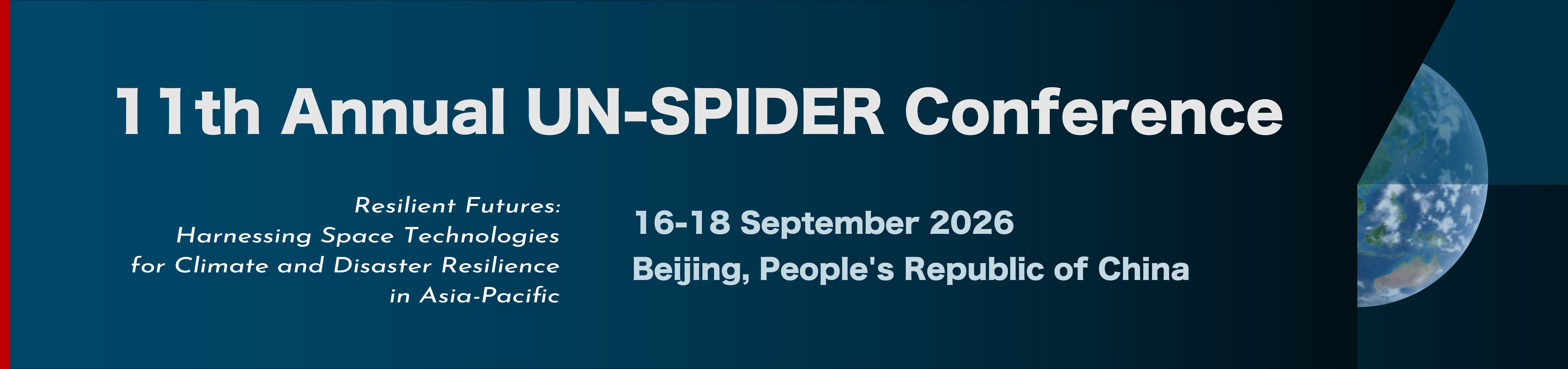
Resilient Futures: Harnessing Space Technologies for Climate and Disaster Resilience in Asia-Pacific
Beijing, People's Republic of China, 14-18 September 2026

![]()