The step-by-step procedures below are for ENVI version 5.
(Click here to access step-by-step instructions for Envi 4.8.)
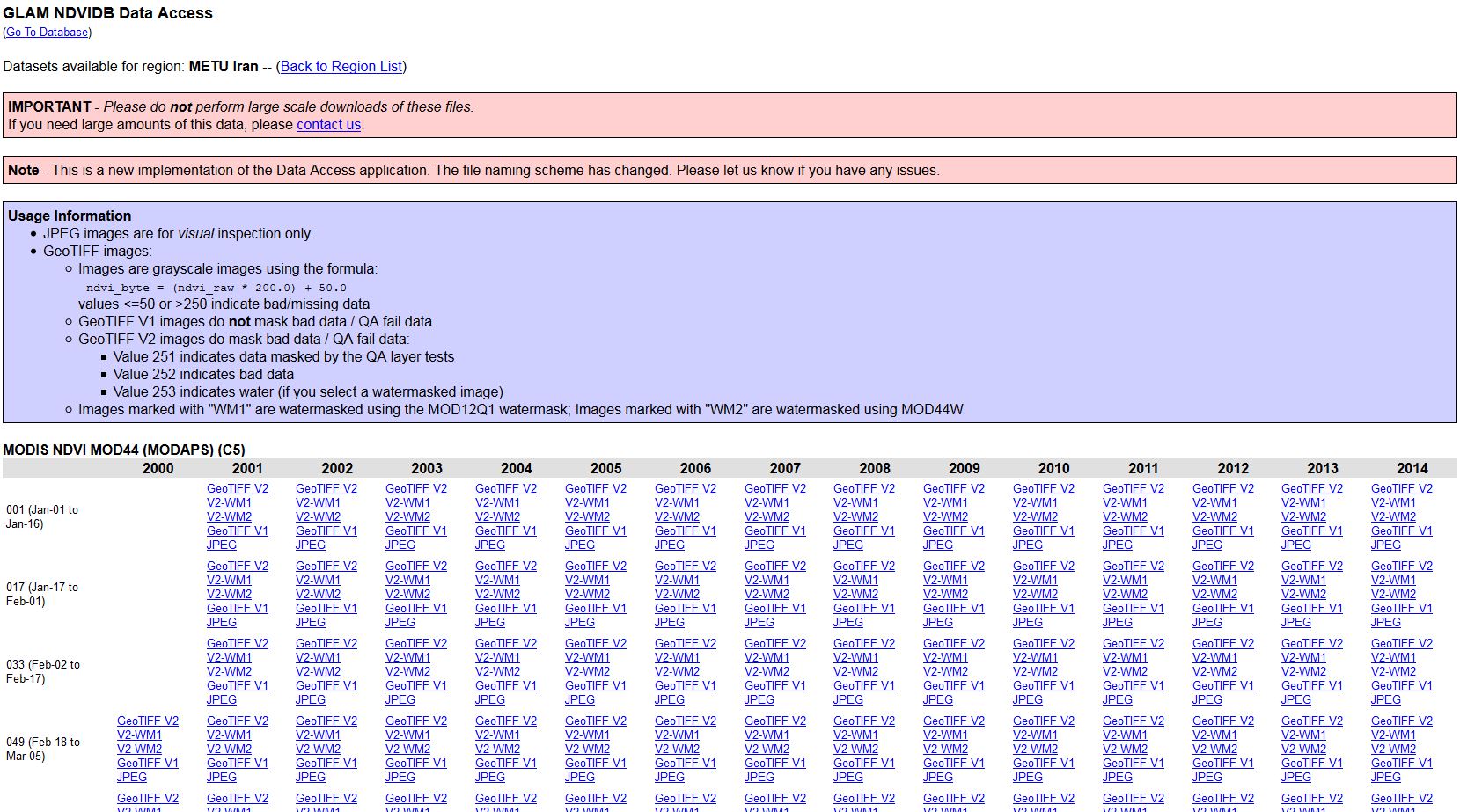
Two-weeks normalized Differenced Vegetation Index (NDVI) composits based on 250m MODIS data are freely available for download from the MODIS/NDVI Time Series Database from the Global Agriculture Monitoring (GLAM) Project provided via the website of Geographic Department of Maryland University. The Data Access App provides easy access to the data for different regions including Iran (cf. figure below). the Maximum Value Compositing (MVC) procedure was applied to derive the two-weeks composits. The resulting geotiff images are greyscale images using the formula ndvi_byte = (ndvi_raw * 200.0) + 50.0. Values below or equal 50 or larger than 250 indicate bad/missing data, which are masked in the geotiff V2 images. Additionally, two products come with a water mask: V2-WM1 using the MOD12Q1 watermask, and V2-WM2 using the MOD44W watermask; in both cases the value 253 indicates water.
Read more about the country background and test site at the bottom.
In this practice it is recommended to compare two months in the time span from 2000-2013. Here we show the procedure for one month. In this case it is for May, from 2000-2013. May and June are the month with maximum vegetation growth in the study area in Iran. In other regions the months have to be selected according to the local phenology.
Step 1: Recalculating from MVC values to NDVI value range
Step 2: Layer Stacking
Step 3: Resizing the NDVI-MVC images to the study area
Step 4: Masking out data with the study area
Step 5: Masking out ‘not vegetation’ data
B. Calculate Vegetation Condition Index (VCI)
Step 6: Compute VCI
Step 7: Visualization
Step 8: Compute Statistics
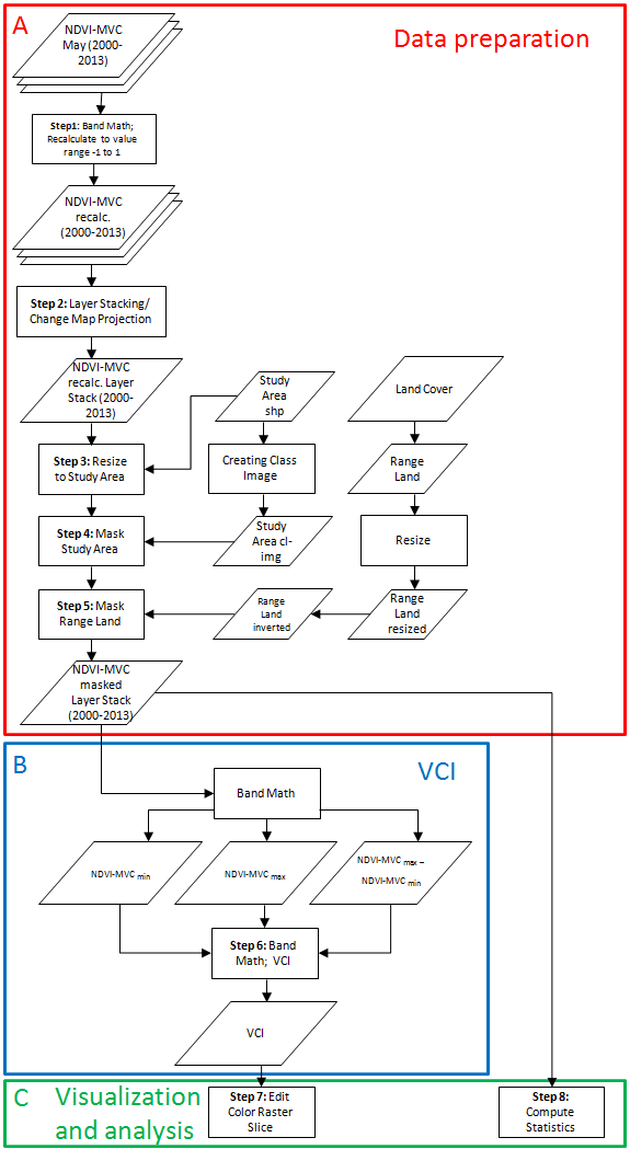
Flowchart of the process chain in ENVI 5.0
Step 1: Recalculating from MVC values to NDVI value range
- As mentioned above, the two weeks NDVI composits are available as 8-bit unsigned integer greyscale images, i.e. the values are ranging from 0-255. However, the standard values for NDVI are within a range from -1 to 1. Therefore, the provided two-weeks NDVI composits have to be recalculated using the formula (ndvi_byte-50)/200. In Envi, the tool for this is called ‘band math’.
- Attention: The current data format of the images is ‘byte’, i.e. the values are integers without digits behind the decimal point. To use the NDVI value range the data format has to be converted to ‘float’, which allows for decimal digits. Therefore, in the following formula the expression ‘float’ is used.
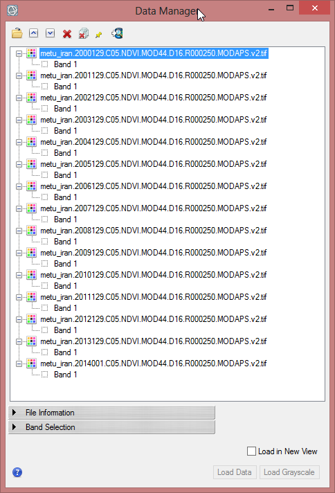
- Open the NDVI-MVC-images from 2000-2013 in the ENVI Data Manager. The images do not have to be displayed.
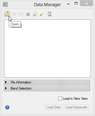
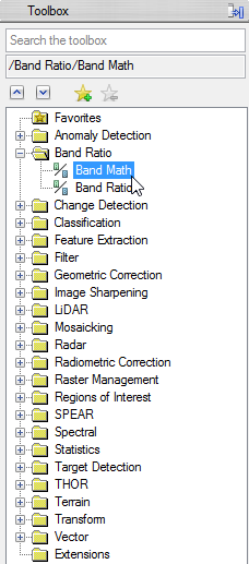
- Enlarge the folder ‘Band Ratio’ in the ENVI Toolbox and double click on ‘Band Math’
- In the Band Math Window write ‘float((b1)-50)/200’ below ‘Enter an Expression:’
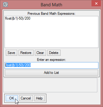
- Click ‘Add to list’, so the expression is stored for this session. When you click on ‘Save’, you can store your expressions on your local drive and can use it in the next session via ‘Restore’.
- Click ‘OK’ to go on with the Band Math calculation.
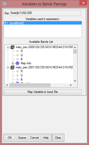
- Now you have to match the right band to the variable in the expression. Click at first on ‘B1 – [undefinded]’ so it is blue shaded. Now choose the one band from the NDVI-MVC from the year 2000. With this you match the expression to a band.
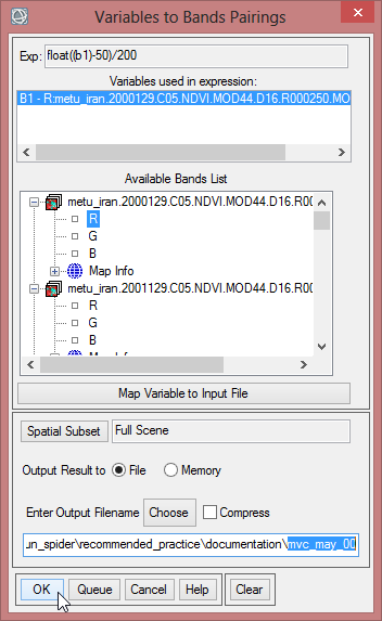
- Save this file as ‘mvc_may_00’.
- Repeat this step, but go on with a band from the year 2001 when matching and so on, until you have finished with the band from 2013 and saved it as ‘mvc_may_13’.
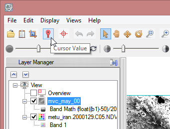
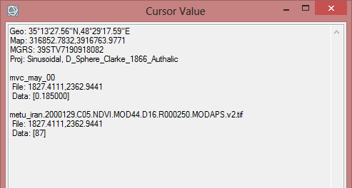
- To check the data you can display the calculated images in ENVI by drack and drop from the Data Manager into the imaging window. Then click on the icon for curser values in the toolbar above. Now move the mouse over the image. In the Cursor Value window you see the values for each pixel. It should be in the range from 0.000000 to 1.010000.
Step 2: Layer Stacking
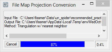
Now you have 13 images, each containing one band with NDVI-MVC values for the one month. For a better and faster proceeding a ‘Layer Stacking’ is used. To continue with the further proceeding it is necessary to have the same Map Projection for all files. In this case, the data shall have the projection Geographic Lat/Lon WGS 1984. Thus, the projection of the NDVI-MVC images must be changed. Both stacking and reprojection will be processed in one step.
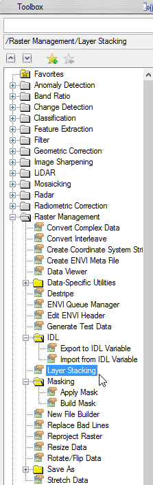
- Enlarge the folder ‘Raster Management’ in the Toolbox. Double click on ‘Layer Stacking’
- In the ‘Layer Stacking Parameters’ window click on ‘Import File…’ to load the calculated images. Choose all of them so they are all blue shaded. Click ‘OK’
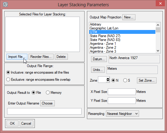
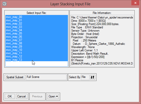
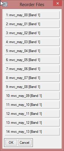
- To check the order of the files click on ‘Reorder Files…’. The first band should start with ‘mvc_may_00’. When the order is not correct, reorder them by drag and drop. Click ‘OK’.
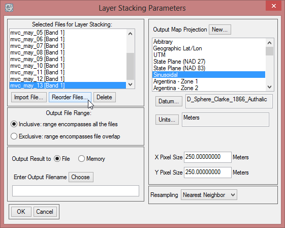
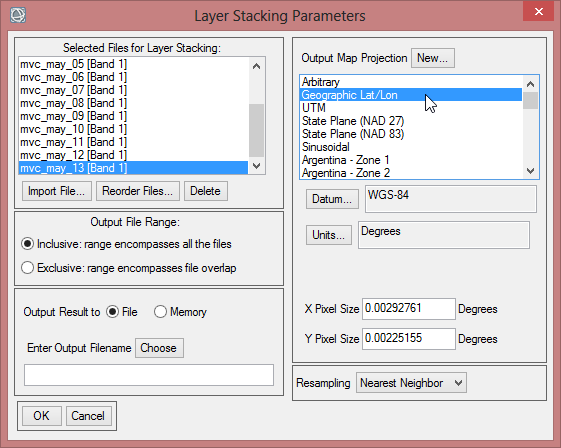
- On the right side of the ‘Layer Stacking Parameters’ you find a section to change the ‘Map Projection’. Click on Geographic Lat/Lon.
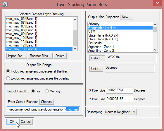
- Save the layer stack as ‘mvc_may’, which contains now all May images for the time span from 2000-2013.
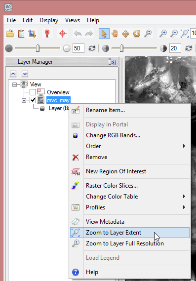
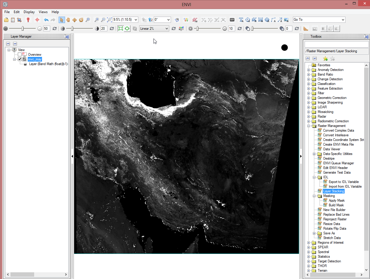
- Computing a layer stack can take some minutes. When it is finished, you can display your result in ENVI.
Step 3: Resizing the NDVI-MVC images to the study area
It is recommended to reduce the amount of data to decrease the time for computing. The test site covers five provinces in Iran (cf. maps 'In Detail'). So a shapefile which represents the provinces will limit the data.
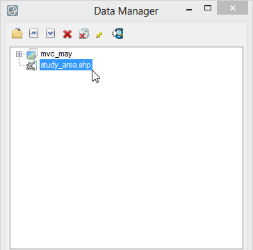
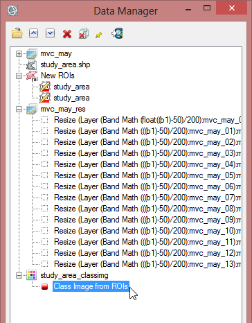
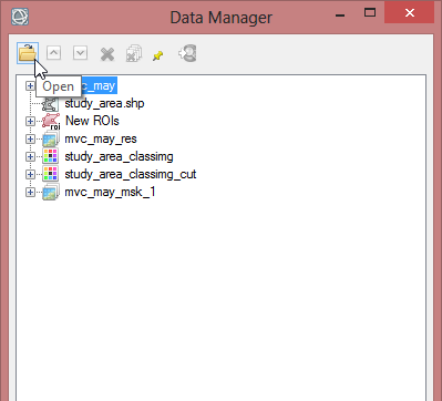
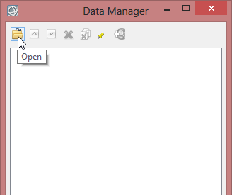
- Before going on you can clear the ‘Data Manager’ for a better overview. Just keep ‘mvc_may’ in the ‘Data Manager’, because the following steps require an associated file.
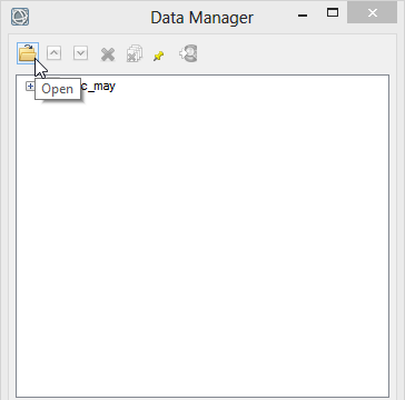
- Click on ‘Open’ in the ‘Data Manager’. Load the shapefile study_area.shp.
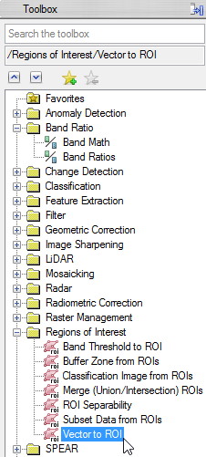
- Go to the toolbox and enlarge the folder ‘Regions of interest’. Double click on ‘Vector to ROI’.
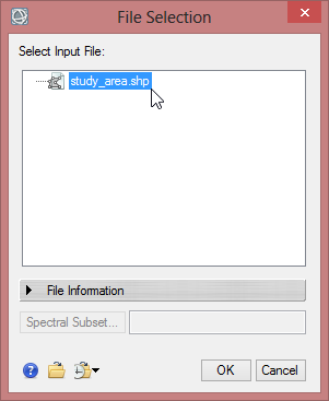
- Click on the shapefile you have loaded and then ‘OK’.
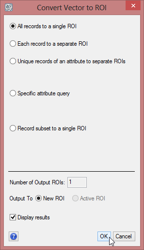
- In the next window ‘All records to a single ROI’ must be checked. The rest keep in default. Click ‘OK’.
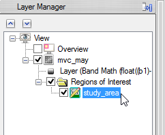
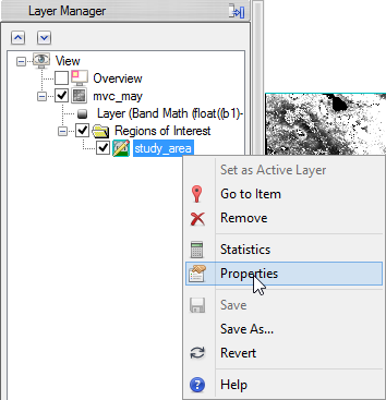
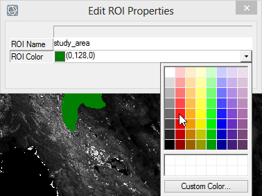
- When you display your Region of Interest you can change the colour of the shapefile via right click on the name in the ‘Layer Manager’. Choose ‘Properties’ and select a colour.
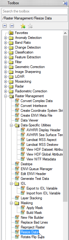
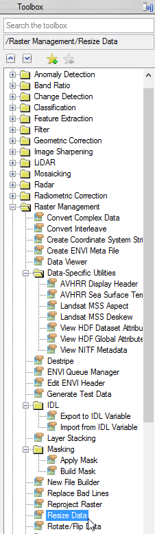
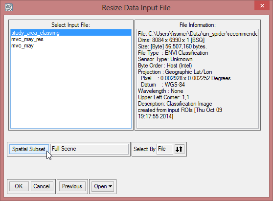
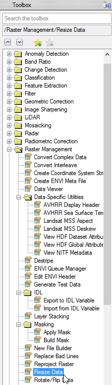
- Now to bring the size of the NDVI-MVC images to the size of the study area, choose ‘Resize data’ in the ‘Raster Management’ of the ‘Toolbox’.
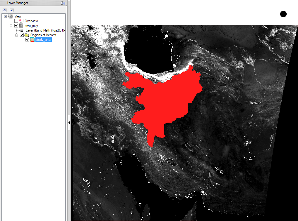
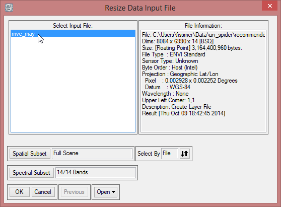
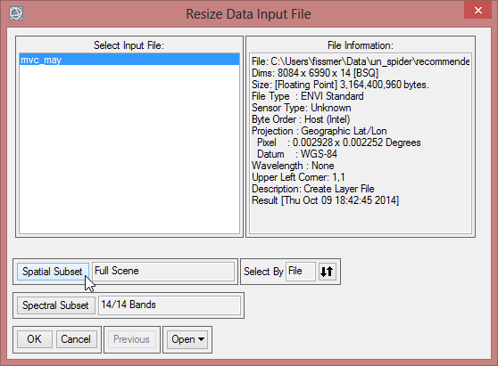
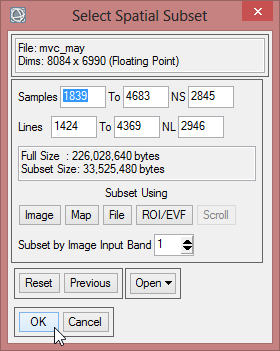
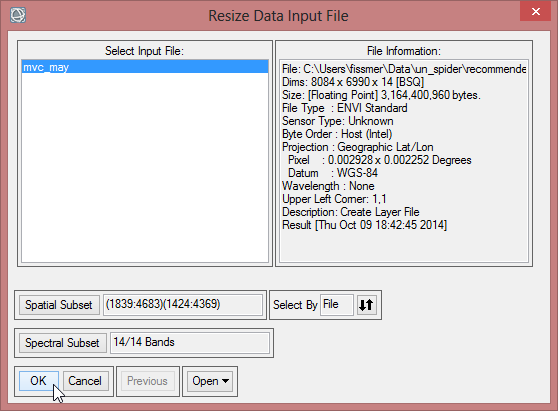
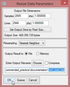
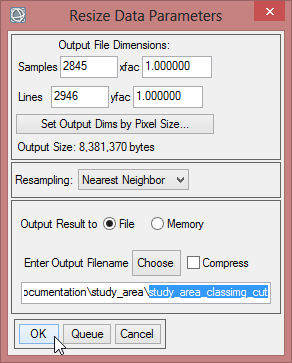
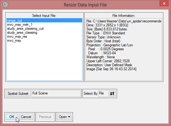
- The ‘Resize Data Input File’ window appears. There choose mvc_may. Click then on ‘Spatial Subset’. There click on ‘ROI/EVF’ and after that you choose study_area as the file you use for resizing. Confirm with ‘OK’ three times until you are asked for the ‘Resize Data Parameters’. Keep the default settings and give the output the name ‘mvc_may_res’.
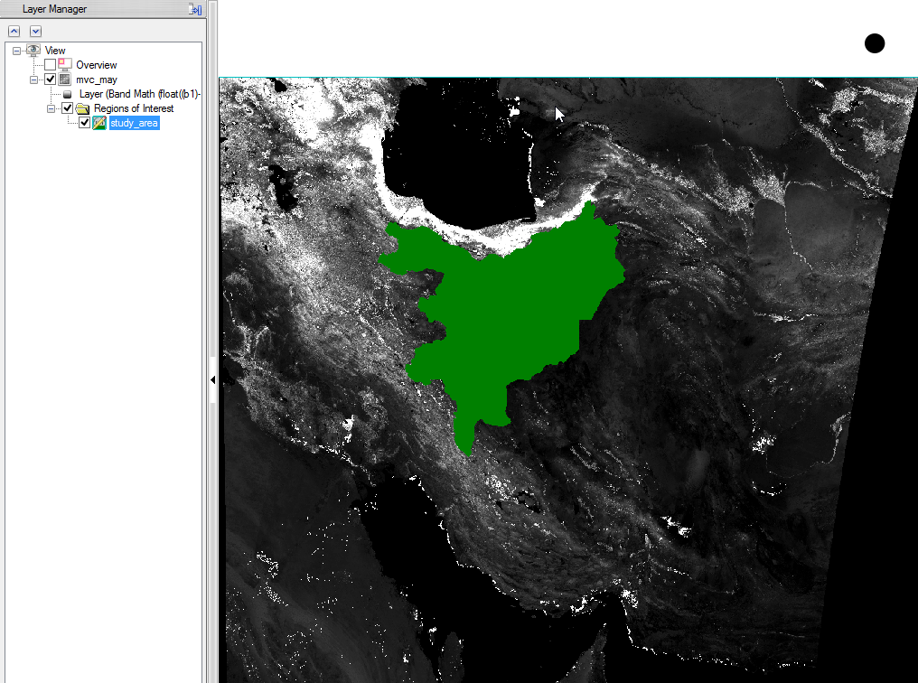
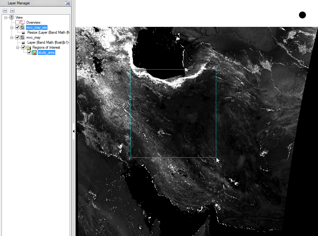
- You can check the result and see if the resized image fits to the outlines of the Region of Interest.
Step 4: Masking out data with the study area
The Region of Interest outlines the study area, but the image contains the pixels, which are in the Region of Interest, but out of the polygon. So the area out of the polygon has to be masked out.
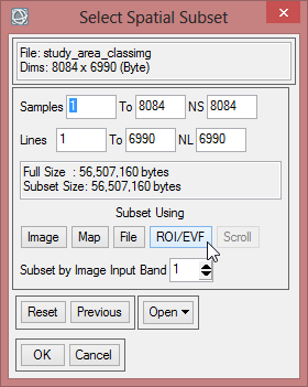
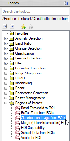
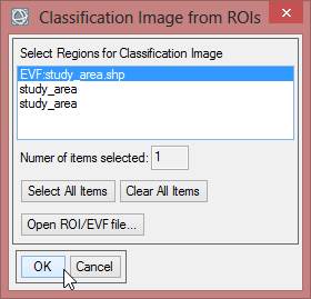
- In the ‘Region of Interest’ section of the toolbox click on ‘Classification Image from ROIs’.
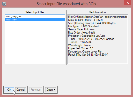
- Now you have to select a file which should be associated with the ROI. Choose mvc_may and click ‘OK’.
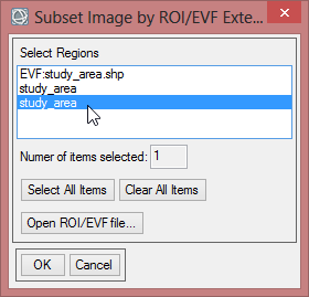
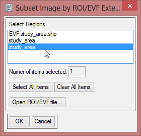
- Select ‘EVF:study_area.shp’ as the region for the classification image. Confirm with ‘OK’. The EVF-file is automatically created when you build a class image from a shapefile.
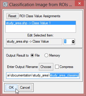
- Save the class image file as ‘study_area_classimg’ and click ‘OK’.
To use the class image as a mask, it needs to have the same size as the file the masking is based on.
- Open the ‘Resize’ tool.
- Choose ‘study_area_classimg’ as input file and click on ‘Spatial Subset’.
- Click on ‘ROI/EFV’ , select study_area and confirm with ‘OK’ three times.
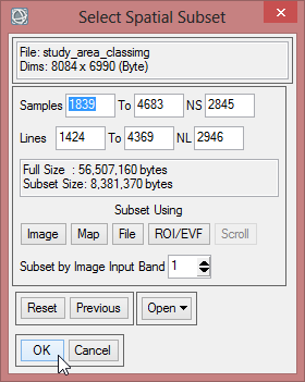
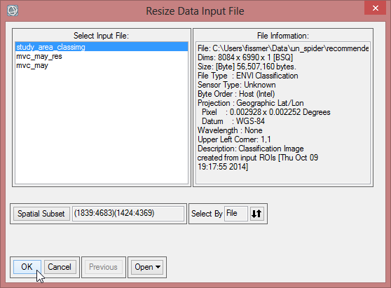
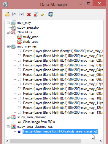
- Save the file as ‘study_area_classimg_cut’ and click ‘OK’.
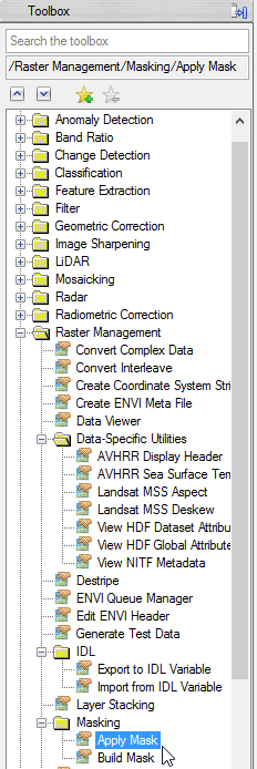
- Go to the ‘Masking’ Folder in the ‘Raster Management’ section in the Toolbox.
- Select ‘mvc_may_res’ as input file.
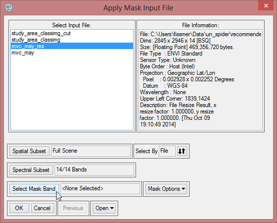
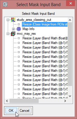
- Click on ‘Select Mask Band’ and choose the cut class image. Confirm with ‘OK’.
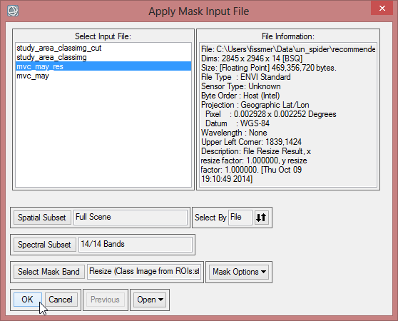
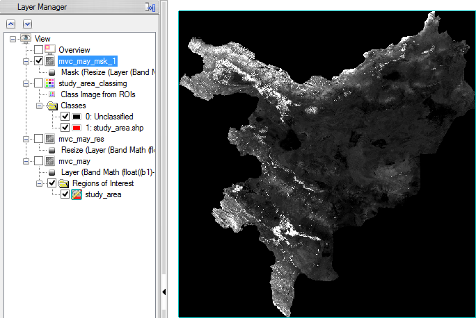
- Save the masked image as ‘mvc_may_msk_1’.

- Now you can check the masked image in the viewer. There shouldn’t be any data displayed outside of the study area.
Step 5: Masking out ‘not vegetation’ data
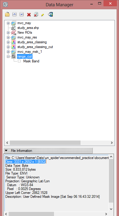
The purpose of this study is to monitor impacts of meteorological drought on natural vegetation, which consists on the classes rain fed, range land and forest. In this procedure only the class range land is used. So the focus is only on areas which represent the class range land. The raster file range_cut consists of pixel values, which represent range land (0) and not range land (1). In the next step all data will be excluded from the NDVI-MVC image, that is not part of the class range land.
But at first the values of the pixels have to be inverted. When applying a mask in ENVI, the ‘0’ values are masked out. To match the pixel values in the present case a conversion is needed.
- Open the range_cut raster file in the ‘Data Manager’
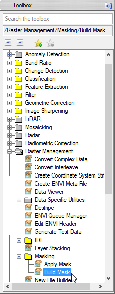
- Go to ‘Build Mask’ in the toolbox and click on it.
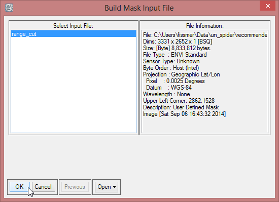
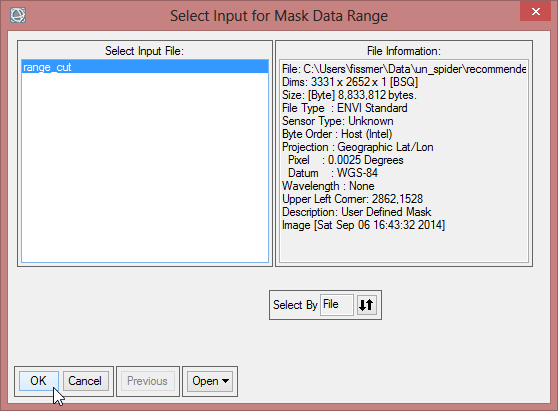
- Choose range_cut as input and confirm with ‘OK’.
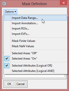
- In the ‘Mask Definition’ choose ‘Import Data Range…’, where range_cut is the input file again. Click ‘OK’.
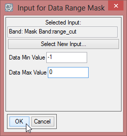
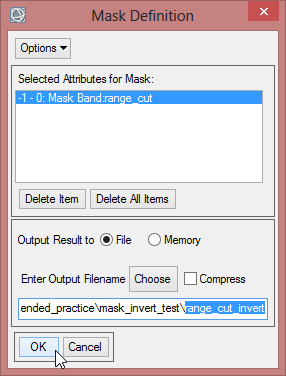
- Now define the ‘Data Min Value’ and the ‘Data Max Value’. With a new data range from -1 to 0 you invert the mask values. Confirm with ‘OK’.
- Save the mask as ‘range_cut_invert’.
- Load ‘range_cut’ and ‘range_cut_invert’ in the ENVI data viewer. Use the function ‘Curser Value’ to compare the pixel values.
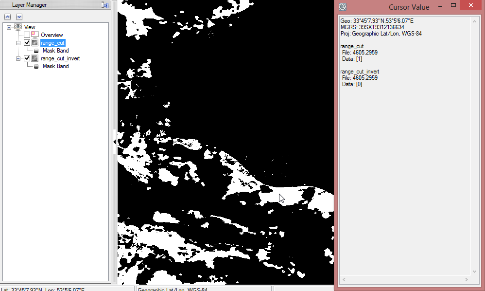
The next step to cut cut out the areas, which are not range land, is to match the properties of the ‘range_cut_invert’ file with the ‘mvc_may_msk_1’ file
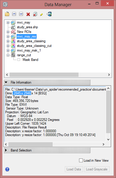
- Open the ‘range_cut_invert’ raster file in the ‘Data Manager’
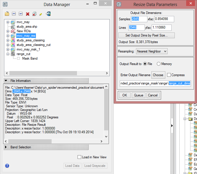
- Click on ‘File Information’ below to see the dimensions (Dims) of the raster file. You will note, that it has more samples and lines than the ‘mvc_may_msk_1’ file. The Pixels size is different as well. To match the Dims and the pixel size to the NDVI-MVC image, and the associated masking, the ‘range_cut_invert’ has to be resized. Before you begin with resizing, click on ‘mvc_may_res’ or on mvc_msk_1 to show the Dims of this image. This will be the output values of the resized range cut.
- Open ‘Resize Data’ in the Toolbox.
- Choose ‘range_cut_invert’ and click ‘OK’.
- Enter in the ‘Resize Data Parameters’ the values of ‘Samples’ and ‘Lines’ according to the Dims of ‘mvc_may_res’
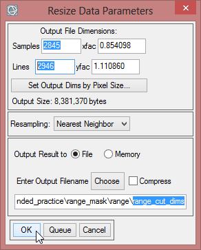
- Save the resized file as ‘range_cut_dims’.
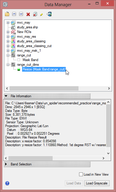
Now the file has the same dimensions and the same pixel size. It can be used as a mask.
- Click on ‘Apply Mask’ in the ‘Masking’ folder in the ‘Raster Management’ in the Toolbox.
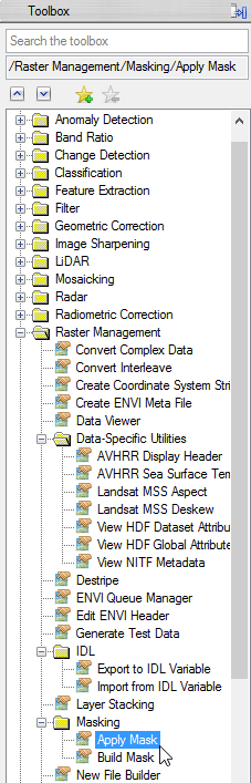
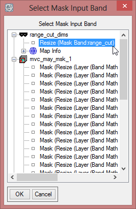
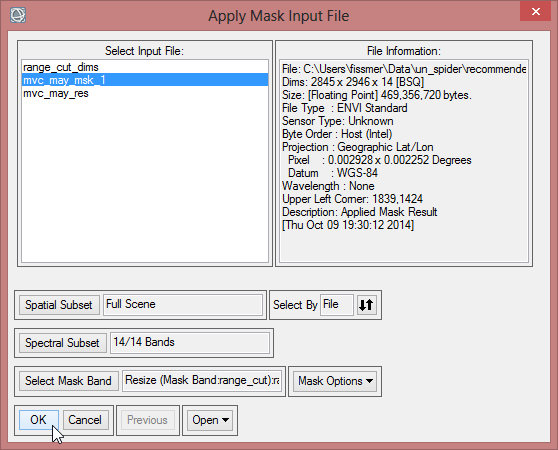
- Choose ‘mvc_may_msk_1’ as input file and click on ‘Select Mask Band’ below.
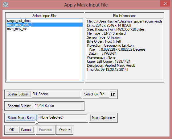
- Select range_cut_dims and confirm three times with ‘OK’.
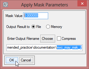
- You can compare your results.
B. Calculate Vegetation Condition Index (VCI)
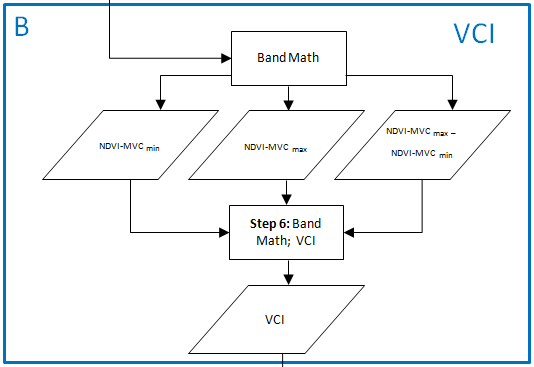
Step6: Compute VCI
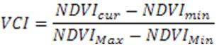
The VCI is calculated by three values: The NDVIcur from a certain month, the NVDImin and the NDVImax.
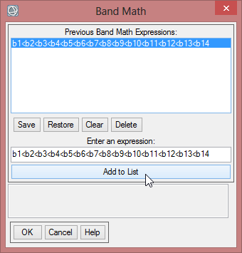
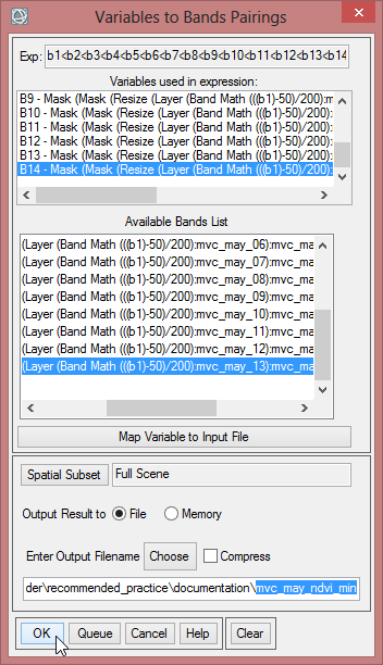
- At first the NVDImin is calculated by following expression in ENVI Band Math: b1<b2<b3<b4<b5<b6<b7<b8<b9<b10<b11<b12<b13<b14
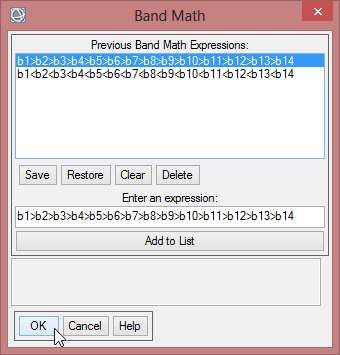
- Open the ‘Band Ratio’ folder in the toolbox and click on ‘Band Math’. Enter the aforementioned expression and confirm with ‘OK’.

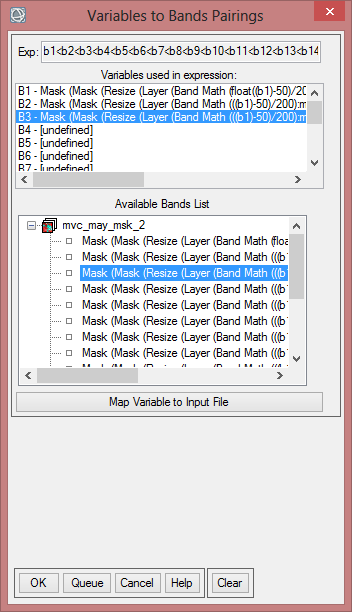
The expression shows 14 variables, that it is working with. Now the variables of the expression have to be matched to the bands of the ‘mvc_may_mask_2’ layer stack.
- Click on the first variable (B1- [undefined]), then select the first band of ‘mvc_may_mask_2’. Go on until each variable is assigned to the correcht band.
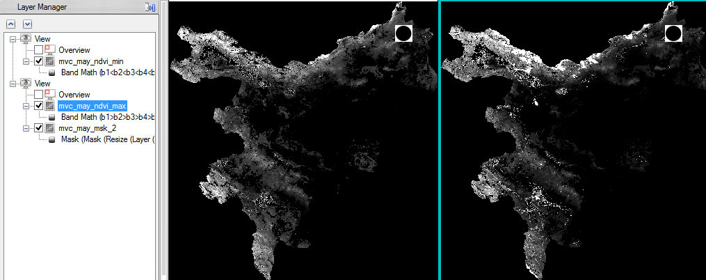
- Save the NVDImin as ‘mvc_may_ndvi_min’
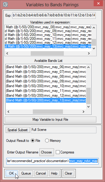
- The next step is to compute the NDVImax with the following expression: b1>b2>b3>b4>b5>b6>b7>b8>b9>b10>b11>b12>b13>b14. Calculate this expression the same way as for NVDImin. Save it as ‘mvc_may_ndvi_max’.
Now the NVDImax-min must be processed.
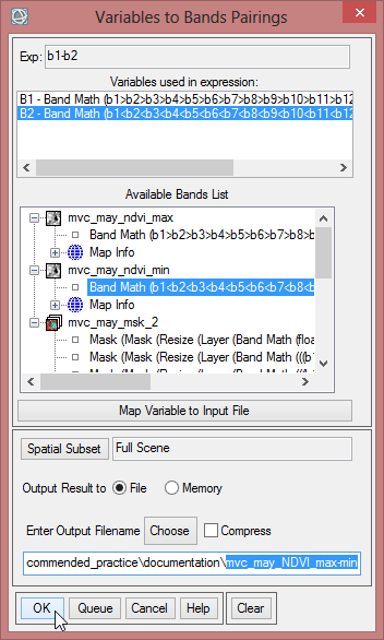
- Choose ‘Band Math’ again. Enter b1-b2. Choose for the first variable the NDVImax. Assign the NVDImin for the second variable.
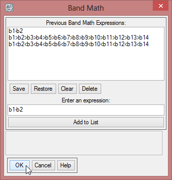
- Save this file as ‘mvc_may_NDVI_max-min’
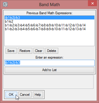
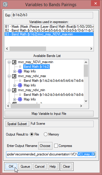
All the items for the VCI are given. With the expression (b1-b2)/b3 the aforementioned formula can be calculated in ENVI. The variable ‘b1’ represents the current month, for that the VCI will be computed. ‘b2’ is the NVDImin while ‘b3’ is the difference of NDVImax and NVDImin.
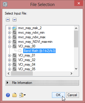
- Be sure, that ‘mvc_may_mask_2’, ‘mvc_may_ndvi_min’ and ‘mvc_may_NDVI_max-min’ are loaded in the ENVI ‘Data Manager’.
- Start a new ‘Band Math’ function with the expression (b1-b2)/b3.
- To calculate for example the VCI for mvc_may_00, choose for the variable ‘b1’ the first band of the layer stack ‘mvc_may_mask_2’. For ‘b2’ select the band from ‘mvc_may_ndvi_min’. The last variable ‘b3’ has to be assigned to the band of ‘mvc_may_NDVI_max-min’. Save the file as ‘VCI_may_00’.
- Go on with all the bands of ‘mvc_may_mask_2’ to calculate the VCI for each month.
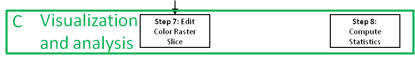
Step 7: Visualization
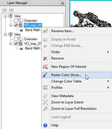
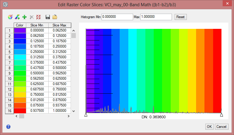
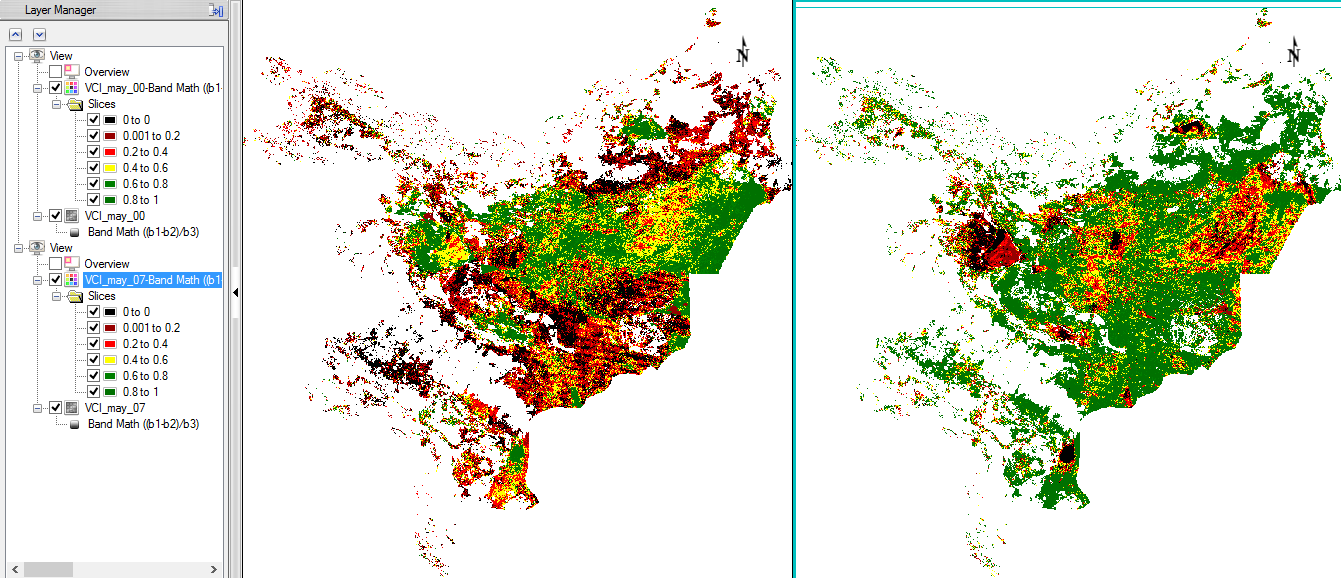
Display some VCI in the data viewer. Load ‘VCI_may_00’ and ‘VCI_may_07’ to compare two months which show a high difference. In the ‘Data Manager’ you can click on ‘Load in New View’, so that the second image will be next to the first data viewer. With the function ‘Raster Color Slices’ classes can be defined and you can assign colours to them. Here values can be excluded in the displaying as well.
- Rightclick on the image name in the ‘Layer Manager’. Select ‘Raster Color Slices’. Choose the band you want to work on.
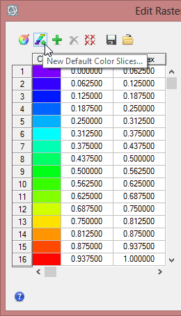
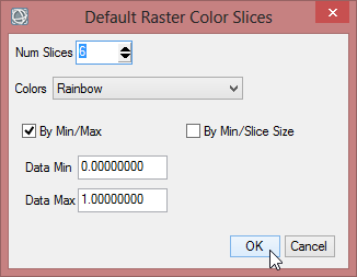
- Click on the button for ‘New Default Color Slices’. Change the number of slices to 6 and confirm with ‘OK’.
- Now change the class break values in the fields ‘Slice Min’ and ‘Slice Max’.
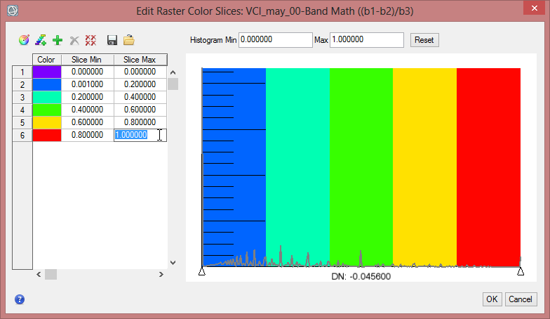
- To define the colours for each class rightclick in the column for ‘Color’ and comfirm ‘Edit Color…’.
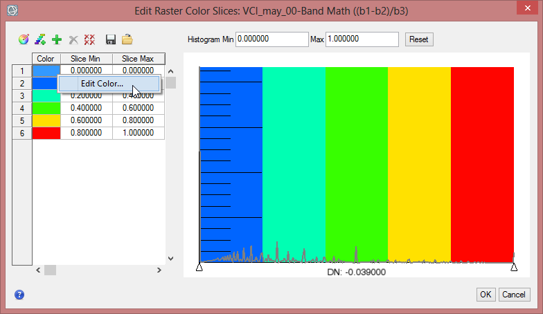

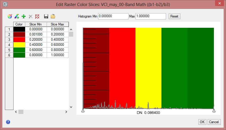
- Repeat the steps for the other VCI image, but make sure you choose the same colours and class break values in both images.
Step 8: Compute Statistics
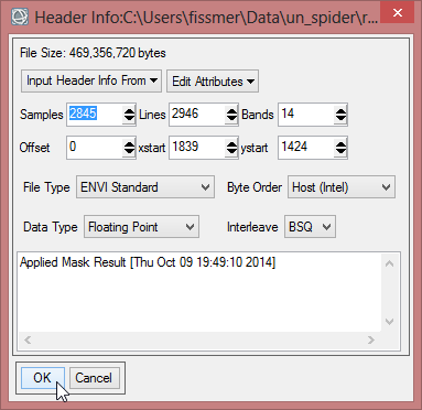
In order to compare average monthly NDVI between 2000 to 2013, statistics of finalized data should be computed. But at first, the ENVI Header must be edited, so pixel with the value ‘0’ aren’t calculated for the statistics.
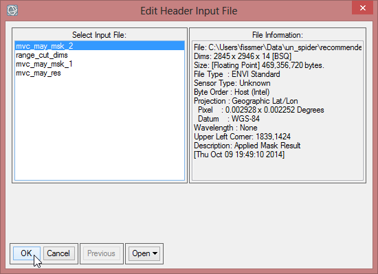
- Go to the toolbox and choose ‘Edit ENVI Header’ in the folder for ‘Raster Management’.
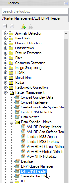
- Select ‘mvc_may_mask_2’ as input file. Click ‘OK’.
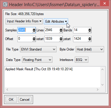
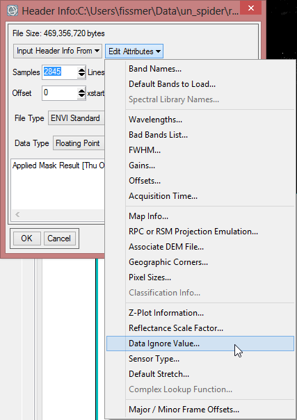
- Open the dropdown menu ‘Edit Attributes’. Choose ‘Data Ignore Value…’.
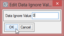
- Enter ‘0’ as Data Ignore Value and confirm with ‘OK’ two times.
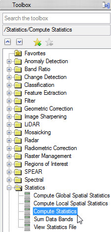
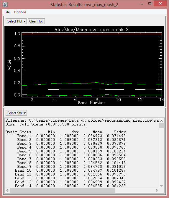
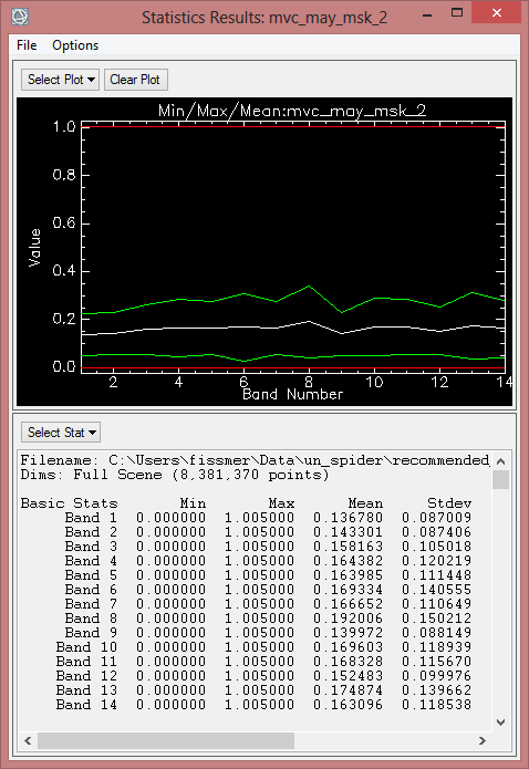
- To compute statistics, enlarge the ‘Statistics’ folder in the toolbox. Click ‘Compute Statistics’.
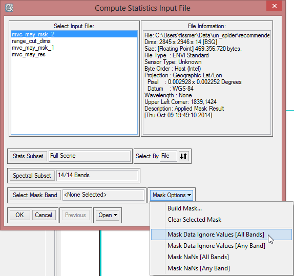
- In the next window choose ‘mvc_mask_2’ as input file.
- Open the dropdown menu of the ‘Mask Options’ and click on Mask Data Ignore Values [All Bands]. This way the value which was defined as ‘Ignore Value’ in the ENVI Header before, won’t be included in the statistics.
- Confirm with ‘OK’.
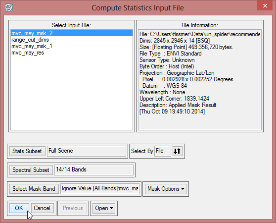
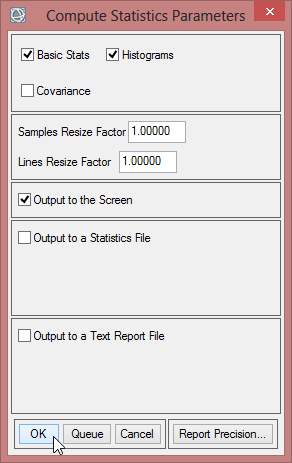
- In the ‘Compute Statistics Parameters’ leave the default settings, but also check 'Histograms' to compute histograms. Click on ‘OK’.
After calculating Indices, the next step is to evaluate which one or ones is the best index for monitoring Drought. This selection generally considers below criteria:
1. Ability of express drought stress on vegetation based on historical observations of time-series MODIS data.
2. Maintaining smooth effect on drought monitoring during the growing season
3. Independent on biophysical land surface characteristics.
Country Background: Iran
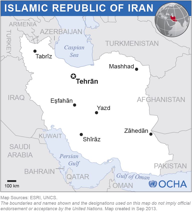
Iran is located in an arid and semi-arid region, between 44º 02 ́ and 63º 20 ́ eastern longitude and 25º 03 ́ to 39º 46 ́ northern latitudes. The country covers an area of about 1.648 million km2. Iran is bordered on the north by Armenia, Azerbaijan, Caspian Sea and Turkmenistan; on the east by Afghanistan and Pakistan; on the south by Oman Sea, Strait of Hormuz and Persian Gulf, and on the west by Iraq and Turkey (cf. figure below).
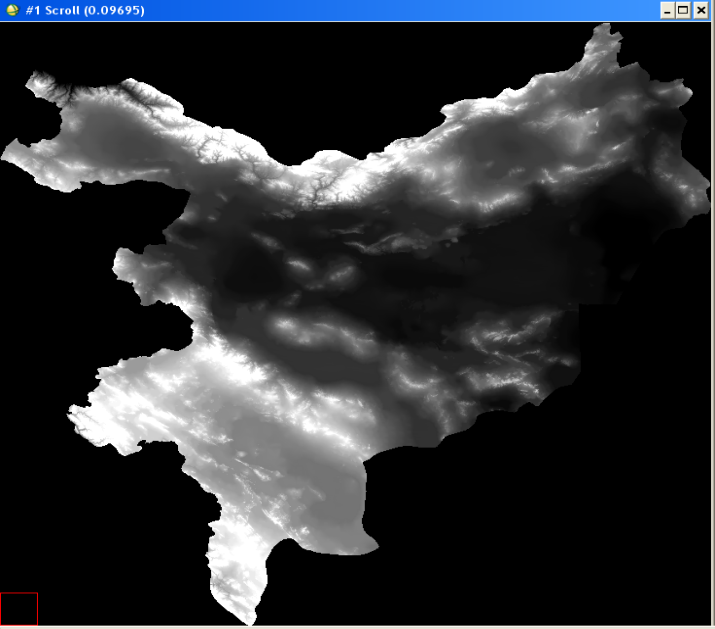
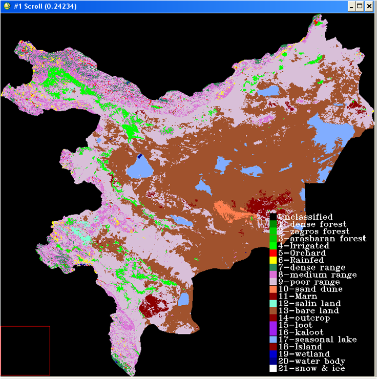
The test site includes the following five provinces in Iran: Alborz, Tehran, Semnan, Qom, Isfahan covering about 250,000km2. The topographic height in the area ranges from 270m to 4,390m. The below images show details of the test site: location of the area within Iran (areas marked purple in the top left image), a Landsat mosaic of the area (top right image), digital elevation model (bottom left) and a land cover map (bottom right).
 |  |
 |  |
Drought impact in Iran
- According to United Nations reports, the cumulative effect of droughts from 1999 to 2001 has seriously affected Iran’s agriculture and livestock production [1].
- In Iran, a three-year drought from 1999 to 2001 has severely affected ten of the country's 28 provinces, leaving an estimated 37 million people (over half the country's population) vulnerable to food and water insecurity.
- Twenty provinces have experienced precipitation shortfalls during winter and spring 2001. According to the statistics of the Ministry of the Interior, water reserves in the country were down by 45% in July 2001.
- In the agricultural sector, Iranian farmers have sold roughly 80% of their livestock, and an estimated 800,000 livestock were lost in 2000 as a result of the drought. An estimated 2.6 million hectares of irrigated lands and 4 million hectares of rain-fed agriculture have experienced the drought’s impact in 2001.
- The most severe drought across the country occurred between 1998 and 2001, with approximately 80% of the country experiencing an exceptional drought.
Bibliography
1. Mokhtari, M.H., (2005). Agricultural Drought Impact Assessment Using Remote sensing: A case study Borkhar district – Iran, M.sc Thesis, ITC University.