The step-by-step procedures below are for ENVI version 4.8.
(Click here to access step-by-step instructions for Envi 5.
Click here to access step-by-step instructions for the free software R Studio.)
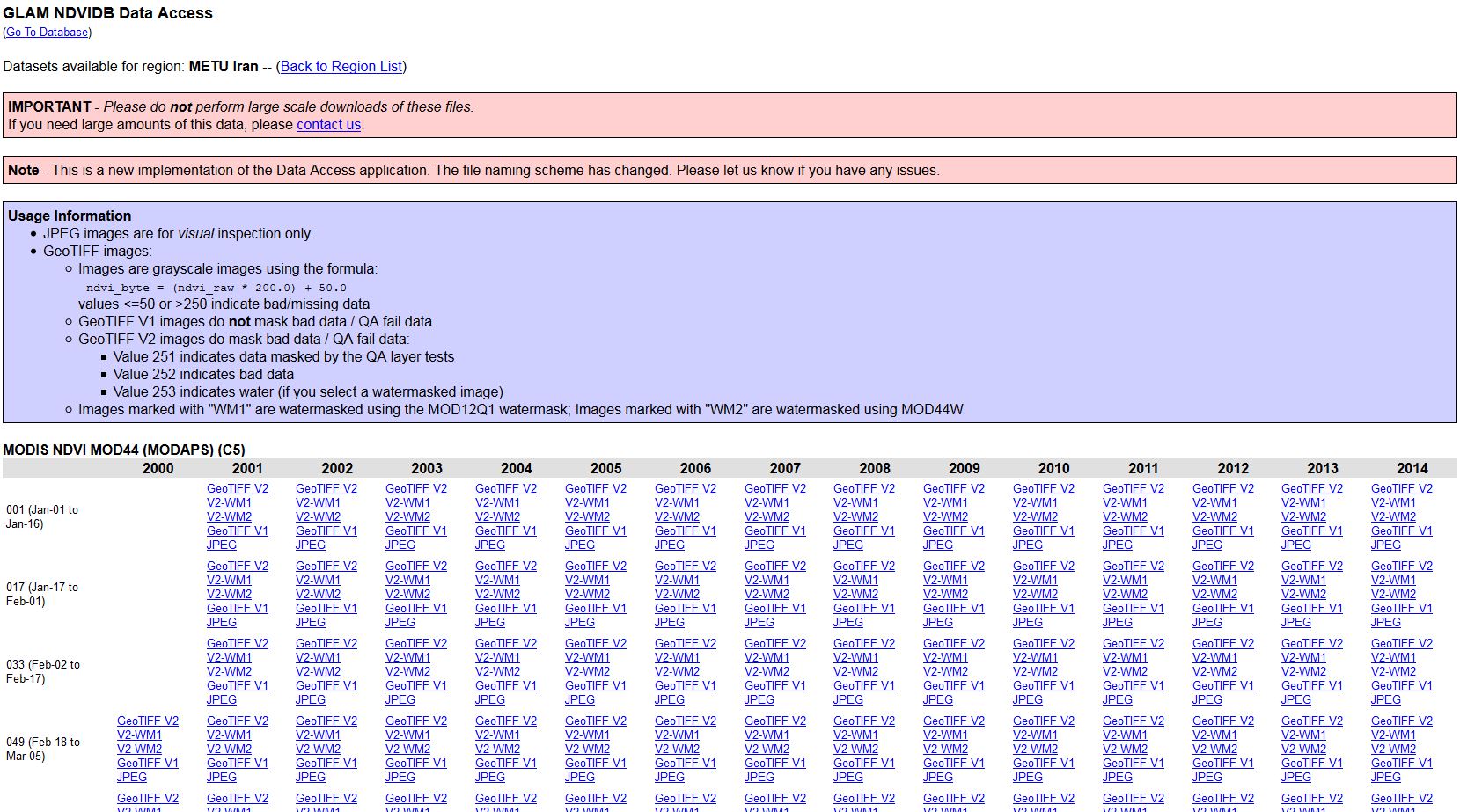
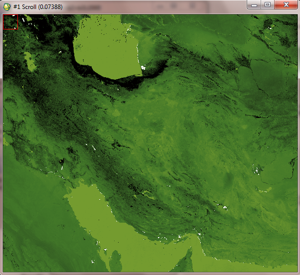
Two-weeks normalized Differenced Vegetation Index (NDVI) composits based on 250m MODIS data are freely available for download from the MODIS/NDVI Time Series Database from the Global Agriculture Monitoring (GLAM) Project provided via the website of Geographic Department of Maryland University. The Data Access App provides easy access to the data for different regions including Iran (cf. figure below). the Maximum Value Compositing (MVC) procedure was applied to derive the two-weeks composits. The resulting geotiff images are greyscale images using the formula ndvi_byte = (ndvi_raw * 200.0) + 50.0. Values below or equal 50 or larger than 250 indicate bad/missing data, which are masked in the geotiff V2 images. Additionally, two products come with a water mask: V2-WM1 using the MOD12Q1 watermask, and V2-WM2 using the MOD44W watermask; in both cases the value 253 indicates water.
In this practice it is recommended to compare two months in the time span from 2000-2013. Here we show the procedure for one month. In this case it is for May, from 2000-2013. May and June are the month with maximum vegetation growth in the study area in Iran. In other regions the months have to be selected according to the local phenology.
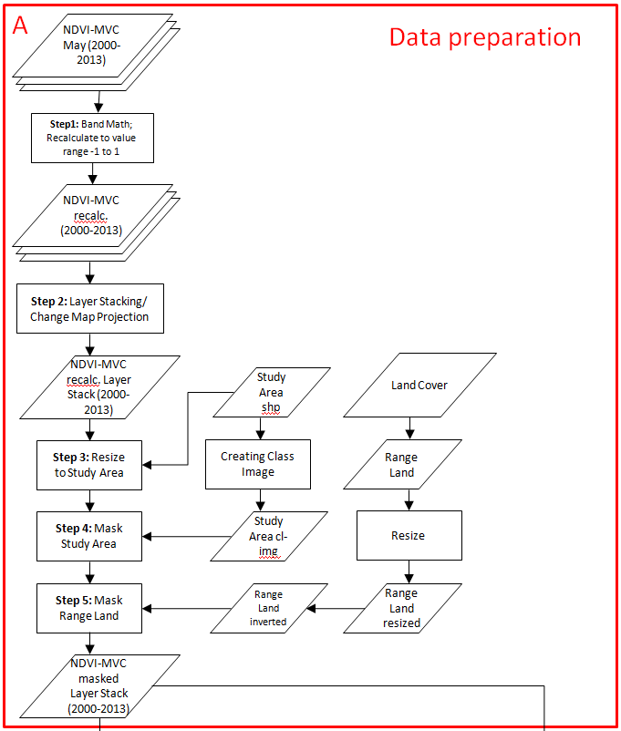
Step 1: Recalculating from MVC values to NDVI value range
Step 2: Layer Stacking
Step 3a: Resizing the NDVI-MVC images to the study area
Step 3b: Change Map Projection
Step 4: Masking out data with the study area
Step 5: Masking out ‘not vegetation’ data
B. Calculate Vegetation Condition Index (VCI)
Step 6a: Compute Statistics
Step 6b: Compute VCI
Step 7: Visualization
Step 1: Recalculating from MVC values to NDVI value range
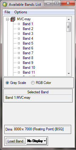
- Input all monthly maximum value composite from 2000 to 2013 using File - Open in ENVI.

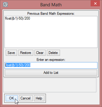
- As mentioned above, the two weeks NDVI composits are available as 8-bit unsigned integer greyscale images, i.e. the values are ranging from 0-255. However, the standard values for NDVI are within a range from -1 to 1. Therefore, the provided two-weeks NDVI composits have to be recalculated using the formula (ndvi_byte-50)/200. In Envi, the tool for this is called ‘band math’.
- Attention: The current data format of the images is ‘byte’, i.e. the values are integers without digits behind the decimal point. To use the NDVI value range the data format has to be converted to ‘float’, which allows for decimal digits. Therefore, in the following formula the expression ‘float’ is used.
- In the Band Math Window write ‘float((b1)-50)/200’ below ‘Enter an Expression:’ (Notice: The band math screenshots below were done in Envi 5.0, but it looks similar in Envi 4.8).
- For more details on the band math operation cf. step-by-step instructions for Envi 5.0 (Step 1: Recalculating from MVC values to NDVI value range)
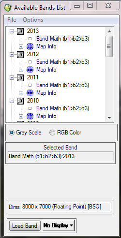
Step 2:Layer Stacking
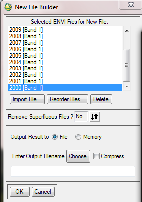
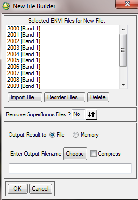
- Create a new raster file including all NDVI MVC data for the whole data range (2000 up to now) using File- Save File as - ENVI Standard
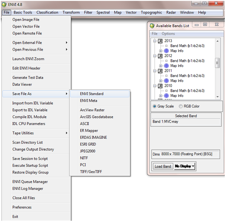
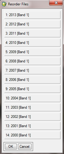
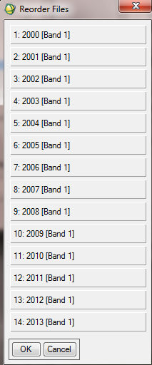
- Import all required NDVI data into the New File Builder window then press Reorder button and sort NDVI data by date and finally save the new file. The result is a new file including all MVCs for May. With the same approach we can make a single file including all MVCs of June.
Step 3a: Resizing the NDVI-MVC images to the study area
It is recommended to reduce the amount of data to decrease the time for computing. The test site covers five provinces in Iran (cf. maps 'In Detail'). So a shapefile which represents the provinces will limit the data.
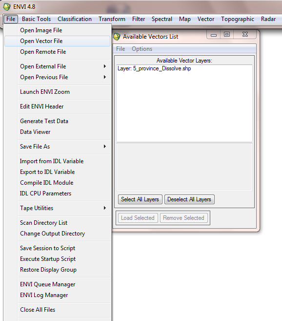
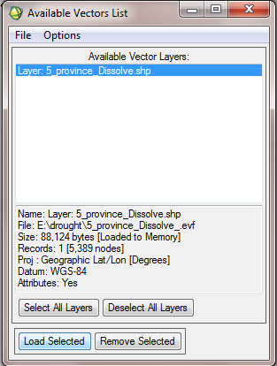
- At the next step, we can resize and cut the generated NDVI composites file based on the boundary of our region of study , so first of all we should open the vector file of the region, with File - Open Vector file, then select the vector file format and browse the file. From available vector list window you can simply load this vector file.
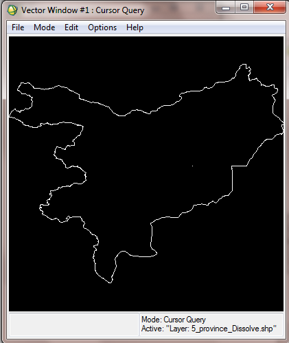
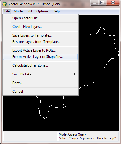
- Then from the Vector Window, open File - Export Active Layer to ROI.
- In the opening window, select the generated MVC file for May and June to associate it with the new ROI.
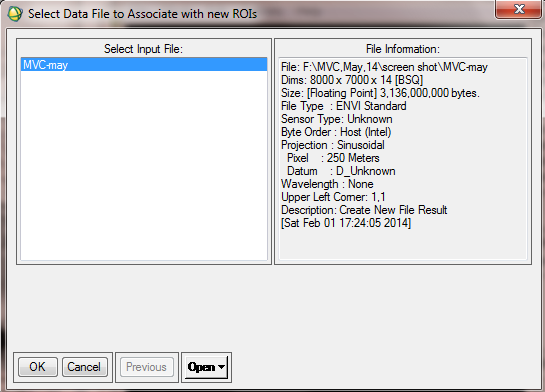
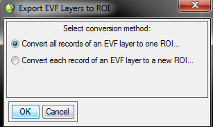
- Finally to make a union ROI, select "convert all records of an EVF to one ROI..."
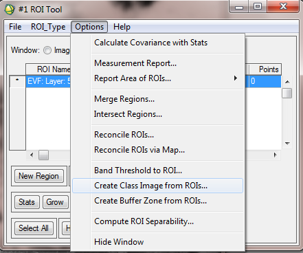
- After overlaying the ROI over the MVC Image, you can adjust the ROI attributes (e.g. color, name…) by opening the ROI tool window from Basic Tools - Region of Interest - ROI Tool.
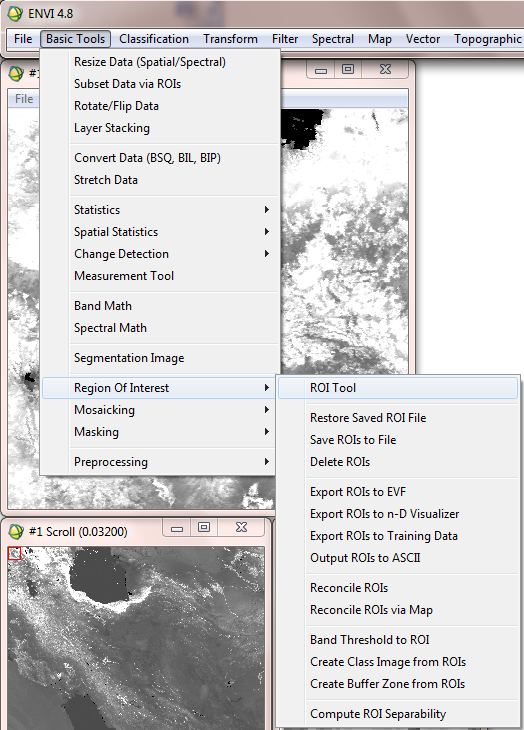
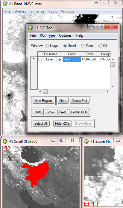
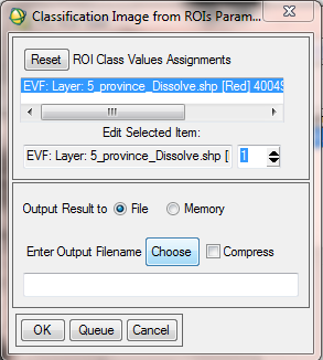
- In order to create a class Images from the ROI (or a raster file from ROI), in the ROI tool window select Options - Create Class Image from ROIs.
- Select the vector layer to classify the MVC Images based on this vector layer.
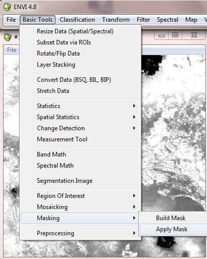
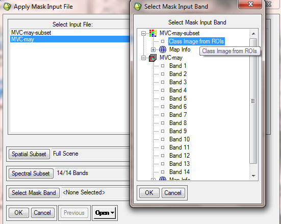
- After creating the Class Image from ROI, we have to apply the mask to create a final masked NDVI image. Therefore from the basic tools menu select Masking and then Apply Mask.
- Then select desired NDVI file.
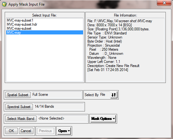
- After that select the Class Image from ROIs as Mask input band.
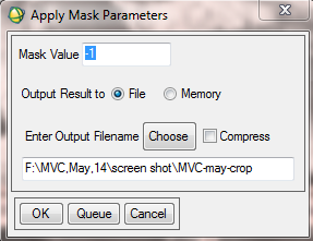
- In Mask parameters window, the mask value should be set to -1, since the minimum value of NDVI is -1. Name the final file as MVC-May-Crop [it means MVC, which is related to May and is cropped, too]. Please note that there are also other solutions to cut or crop a raster file in ENVI.
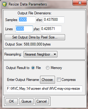
- To decrease the data size and to increase the speed of processing, it is recommended to resize the MVC-crop data. For this purpose from Basic Tools, choose Resize data.
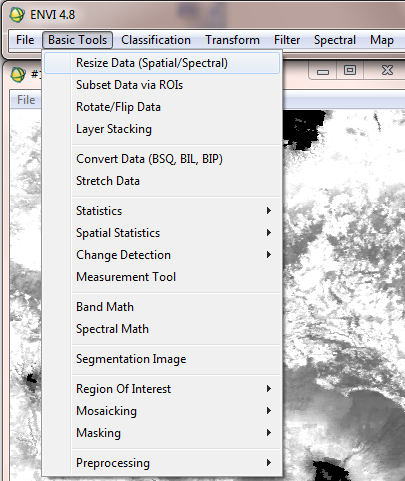
- Then choose the input data file.
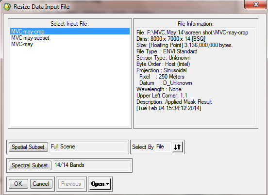
- In the resize data parameters window, set samples and lines according to region of interest. The result of this step is MVC-May-crop-resize raster file.
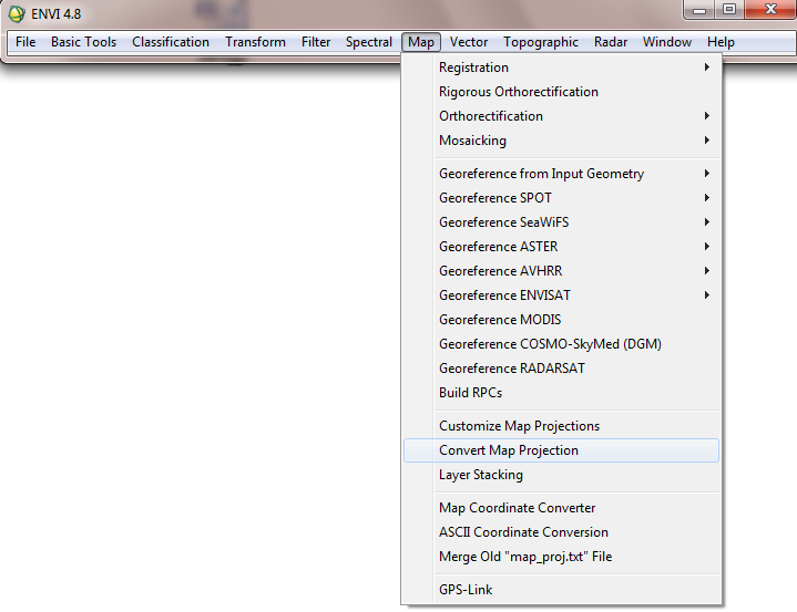
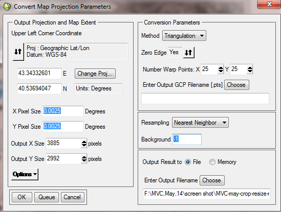
Step 3b: Change Map Projection
- The current projection of data file is sinusoidal. It needs to be converted to Geographic or LatLong projection. In the ENVI Map menu select Convert Map projection.
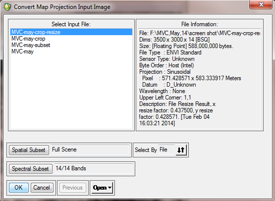
- Then Select Input files e.g. MVC-may-crop-resize.
- In the convert Map projection window, click “change proj”. In the new window, select Geographic Lat/Lon.
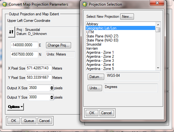
- In the Convert Map Projection Parameters window, set the same values for X pixel size and Y pixel size. For 250 meter MODIS bands you can set 0.0025 for pixel size in degree.
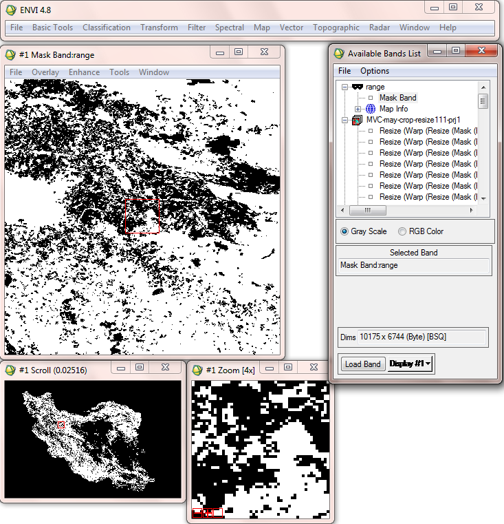
Step 4: Masking out data with the study area
Range land, rain fed and forest are three types of natural vegetation, which were extracted from the available land cover map. In this study area there is no significant forest, so processing continues with range land and rain fed land. IN the below figure the distribution of range land is shown.
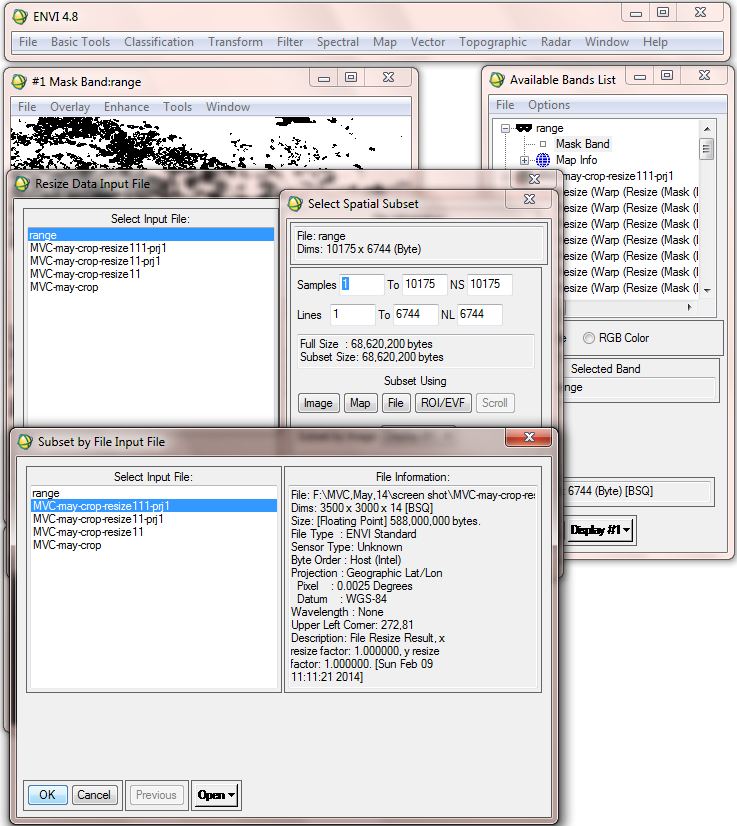
Step 5: Masking out ‘not vegetation’ data
To subset range land, select resize data, choose spatial subset and click file in “select spatial subset” window. Now choose MVC-may-resize-prj, which is the file that the range land subset should be based on. Final result is range-cut.img.
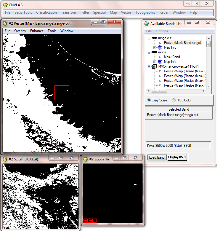
The figure below shows the resized range land based on MVC.
The following figure shows the range land of the sample area.
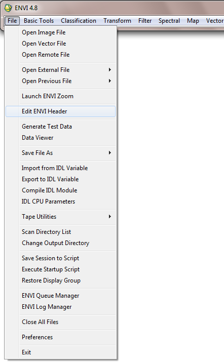
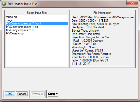
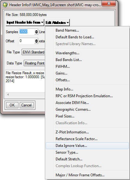
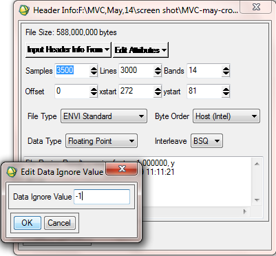
Since the minimum value of NDVI is -1 , the ignore value of MVC data file should be set to -1. So, in ENVI Header, after selection of Input file, in the Edit/attributes tab, click on “data ignore value”, and set -1 in the new window.
B. Calculate Vegetation Condition Index (VCI)
Step 6a: Compute Statistics
(note: in the workflow diagram this is step 8.)
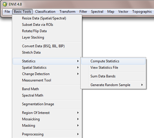
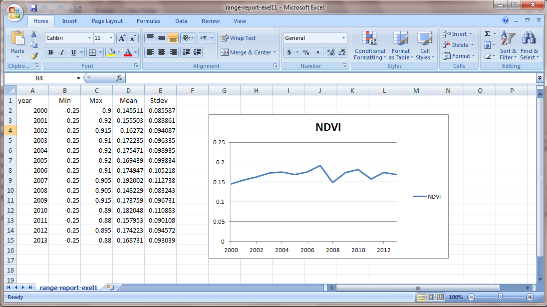
- In order to compare average monthly NDVI between 2000 to 2013, statistics of finalized data need to be computed. To compute statistics, from Basic Tools, select Compute statistics.
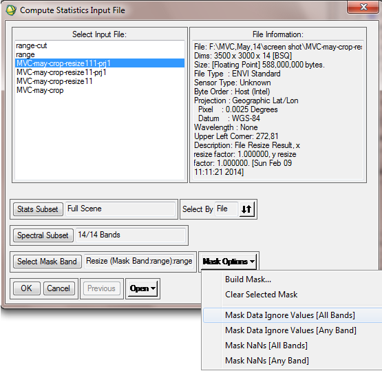
- In the “Compute Statistics Input File” Window, after selecting desired data file, in Mask Option tab, choose “Mask Data Ignore Values [All bands]”, because at a previous step -1 value was set for data ignore value. This operation applies mask value for all 14 bands.
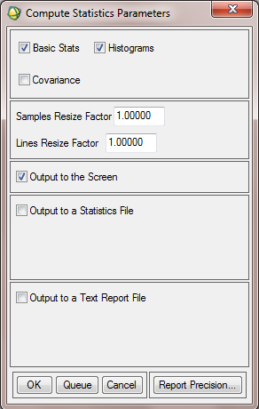
- In the next window, it is possible to choose types of statistical report. Histograms, Basic statistics and covariance are various options.
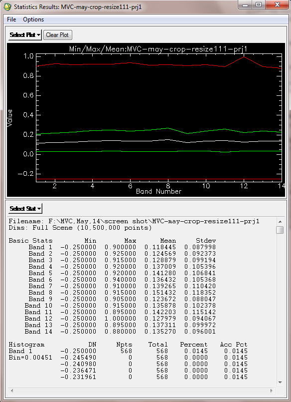
In order to illustrate the drought condition in study area, a line fits to the mean NDVI in period (2000-2013). This constant line is considered as NDVImean,y. The differences between the long-term NDVI mean values and the NDVI values in a specific year is the deviations (DEV NDVI).
DEV NDVI = NDVIi - NDVImean,y
Where, NDVIi is the NDVI value for year i and NDVImean,y is the long-term mean NDVI for the long term period. In fact this line considers as a threshold to determine drought, wet or normal year. When DEV NDVI is negative, it indicates an under normal vegetation condition/health and, therefore, suggests a prevailing drought situation. The greater the negative departure, the greater the magnitude of a drought. In general, the departure from the long-term mean NDVI is effectively more than just a drought indicator, as it would reflect the conditions of healthy vegetation in normal and wet years.
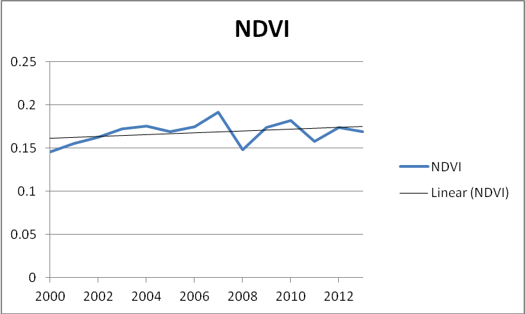
- For the comparison of Mean NDVI values from 2000 to 2013, in Excel software design a graph, the horizontal axis of the graph could be years 2000 to 2013. The vertical axis is the mean values of NDVI from 2000 to 2013 for May.
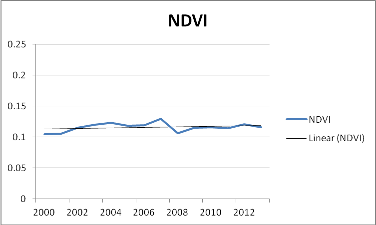
- All processing level from the first stage to the end is performed for June month too. Therefore Mean NDVI from 2000 to 2013 for June is computed with the same algorithm.
Step 6b: Compute VCI
Seasonal and international comparisons of drought areas delineated by the Vegetation Condition Index (VCI) provided a useful tool to analyze temporal and spatial evolution of regional drought as well as to estimate crop production qualitatively. The VCI compares the observed NDVI to the range of values observed in the same period in previous years. The VCI is expressed in % and gives an idea where the observed value is situated between the extreme values (minimum and maximum) in the previous years. Lower and higher values indicate bad and good vegetation state conditions, respectively.
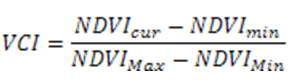
- To compute VCI, at first NDVImin, NDVIMax and NDVIcur need to be computed. NDVImin is defined as minimum value of NDVI in years (2000-2013). So, at first the minimum value of NDVI for each year is computed [since for this case study, MVC for month May and June were used, using b1<b2 expression in ENVI we can estimate the minimum value of NDVI for each year], after that NDVImin from 2000 to 2013 can be computed.
- A month-by-month (May and June) spatial distribution of VCI in the study area during the period (2000-2013) is processed.
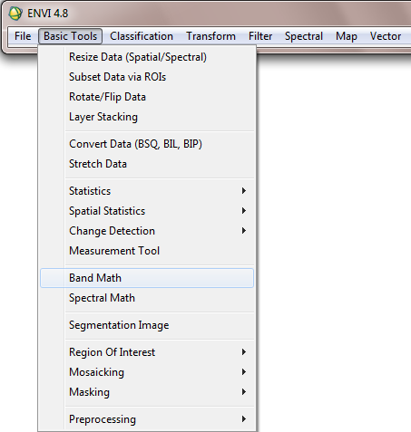
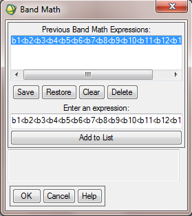
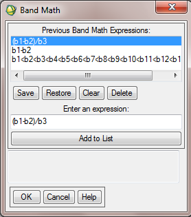
- To compute VCI in ENVI, from Basic Tools, click on Band Math.
- In the opening window, to compute NDVImin type below expression:
b1<b2<b3<b4<b5<b6<b7<b8<b9<b10<b11<b12<b13<b14
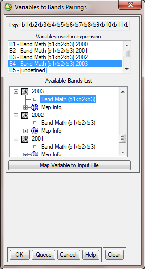
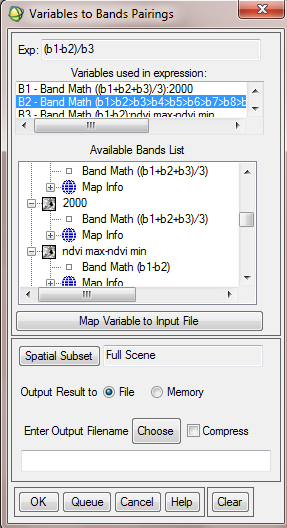
- Then allocate the respective bands to each variable. For example, b1 is allocated to NDVI 2000 or b4 is allocated to NDVI 2003.
- NDVImax and NDVImin are calculated from the long-term record. To compute NDVImax, write below expression in Band math window. Then allocate the maximum value of NDVI for each year to the corresponding variable.
b1>b2>b3>b4>b5>b6>b7>b8>b9>b10>b11>b12>b13>b14
- The next expression is b1-b2= NDVImax - NDVImin
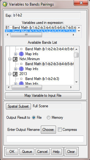
- The final expression to compute VCI is (b1-b2)/b3. b1 is average NDVI of three months (May, June) in each year. So the output includes 14 bands or 14 VCI from 2000 to 2013.
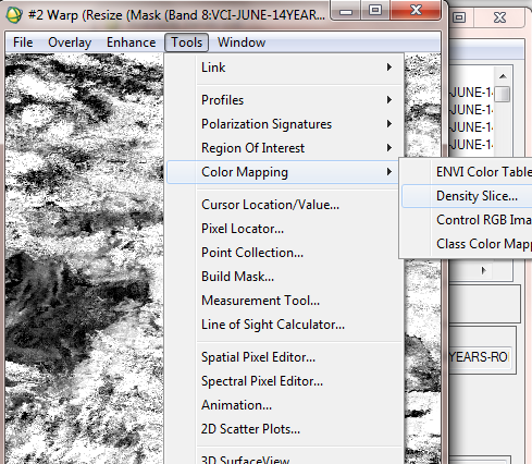
Step 7: Visualization
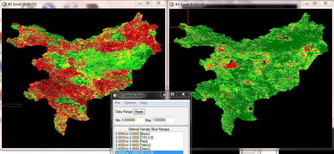
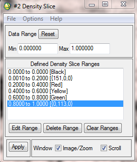
- In order to enhance the colors of the output map, it is recommended to classify the VCI map based on the data range. The data range varies from 0 to 1 (0 showing areas without vegetation and 1 showing areas with dense and healthy vegetation). To perform it from the Tools tab in image window, go to Color Mapping and choose Density Slice.
- In the opening window, it is possible to define the density slice ranges and allocate the desired color for each range.
- In the below figure, the final VCI for May 2000 and May 2007 are compared.