1. Download datasets
For the Recommended Practice the following datasets are needed and can be downloaded from:
Digital Elevation Model (DEM)
Use a DEM with the highest resolution available. Some countries offer openly accessible high-resolution datasets; however, this is not the case globally. Partners such as Airbus can provide commercial, high-resolution data, such as the WorldDEMneo. This dataset offers global coverage and supports modeling at a global scale. For inquiries about WorldDEMneo, please contact Airbus (see Airbus contact).
An openly available and practical alternative is the Copernicus 30 m Digital Surface Model (DSM), which is derived from Airbus’s WorldDEM data. This DEM is used in this practice to demonstrate the feasibility of modeling storm surges using openly accessible elevation data.
For more details on the COP30 DEM see: https://dataspace.copernicus.eu/explore-data/data-collections/copernicus-contributing-missions/collections-description/COP-DEM
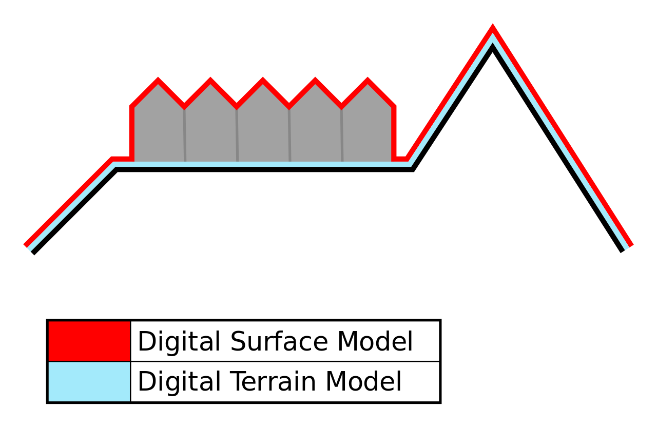
Note: There are two types of Digital Elevation Models:
- Digital Surface Model (DSM): represents the bare-earth surface with all natural and built features (houses, trees, cars,...). This one is preferred for storm surge modelling because it counts in potential barriers against storm surges.
- Digital Terrain Model (DTM): represents only the bare-earth surface without natural and built features
Please note that if a local, more accurate DSM (e.g., WorldDEM Neo) is available, take advantage of this resource.
Shoreline dataset
The shoreline dataset should preferably be with global coverage. If a local, more accurate shoreline vector file is available, take advantage of this resource.
| Dataset | Download |
| Copernicus DEM | Option 1: OpenTopography (quick access, no registration required, see full description below) Option 2: CODE-DE (requires registration) Option 3: Copernicus Data Space Ecosystem (requires registration and approval for CCM DEM/COP DEM data, approval might take a few days) |
| Shoreline from OpenStreetMap | https://osmdata.openstreetmap.de/data/water-polygons.html Download > Format: Shapefile, Projection: WGS84 (large polygons are split) > Download button (see detailed description below) |
Download DEM data from OpenTopography
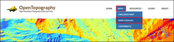
Go to the website: https://opentopography.org/
Click on Data > Data Catalog
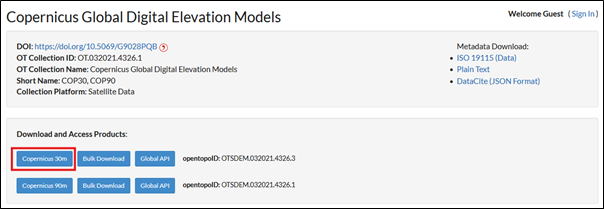
Select Global & Regional DEM and then click on Copernicus Global Digital Elevation Models.
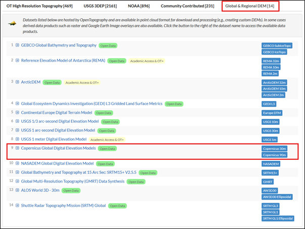
Select the Copernicus 30m DEM for the highest and most feasible resolution available as openly accessible data. The following Figure 4 provides a detailed overview of the available Copernicus DEMs.
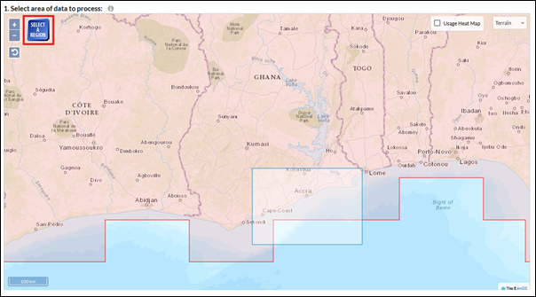
Scroll down to ‘1. Select area of data to process’ and select a region of interest. For our example we use the AOI around Accra, Ghana. Click “select a region” and draw a rectangle.
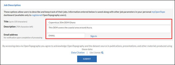
Scroll down and keep the default settings. Under 'Job Description,' define a title for the area and add a description to identify the dataset's content. Enter your email address and submit (Fig. 6).
Check your email for a link to the download section. This process may take a few minutes depending on the dataset's size.
Download the dataset.
(Alternative) Download DEM data from CODE-DE
Alternatively, you can download the DEM data from the CODE-DE.
Go to website: https://explore.code-de.org
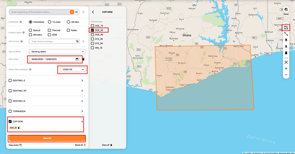
Login or register a new account. Download the data, by selecting the COP DEM and time frame, draw a polygon in the area of interest, click on search and download the desired tiles (Fig. 7).
(Alternative) Download DEM data from Copernicus Data Space Ecosystem (CDSE)
Alternatively, you can download the DEM data from the CDSE.
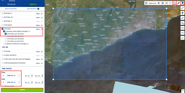
Go to website: https://browser.dataspace.copernicus.eu
Login or register a new account. Then request access to CCM data. After a few business days, you should be able to download the data, by selecting the COP DEM and the time frame, draw a polygon in the area of interest, click on search and download the desired tiles (Fig. 8).
Download "shoreline" data from OpenStreetMap
Go to the following website: https://osmdata.openstreetmap.de/data/water-polygons.html
On this website you find global water polygons that are used for creating our shoreline.
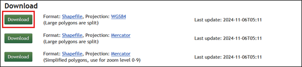
Download the water polygons shapefile dataset with the WGS84 projection (Fig. 9).
Save the DEM and the shoreline dataset in one folder and open QGIS.
2. Load data in QGIS
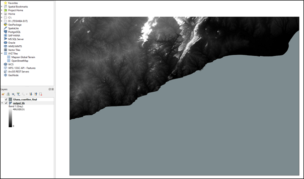
Load the DEM raster file and shoreline vector file in QGIS (Fig. 10).
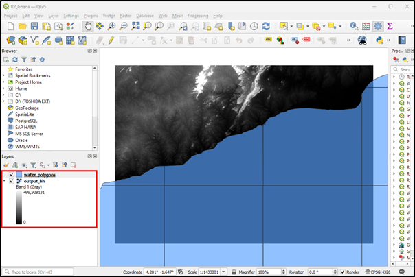
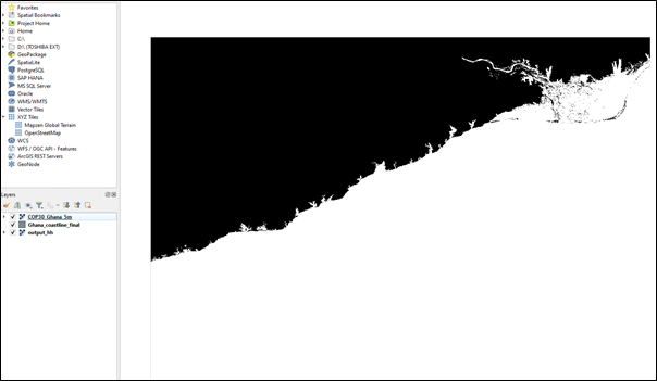
In the background, the loaded Digital Elevation Dataset (greyscale image) is visible (layer name: output_hh); here it is the Copernicus DEM with a 30 m resolution (Fig. 10). The shoreline vector file (layer name: water_polygons) is displayed in transparent blue. When sourced from OpenStreetMap (OSM), this file provides global coverage and appears in separate tiles, encompassing the entire world in the QGIS project. In the next step, the shoreline dataset will be preprocessed to enable further analysis for the chosen region of interest.
3. Preprocessing
3.1 Shoreline
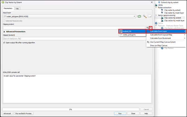
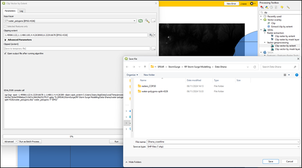
Search for the 'Clip Vector by Extent' function in the QGIS Processing Toolbox. Use the worldwide water polygon layer from OSM as the input layer and select the raster layer as the clipping extent (Fig. 11).
Under 'Clipped (extent),' select a folder and click “save to file” and assign it a name (e.g., Ghana_coastline). You can save it as shapefile (.shp) or as Geopackage (.gpkg). Here it was saved as shapefile. Then click 'Run' (Fig. 12).
A new layer has been created in your QGIS project, displaying only the extent of the selected raster DEM. To maintain a clearer overview, remove the 'water_polygon' layer by right-clicking on the layer and selecting 'Remove Layer'.
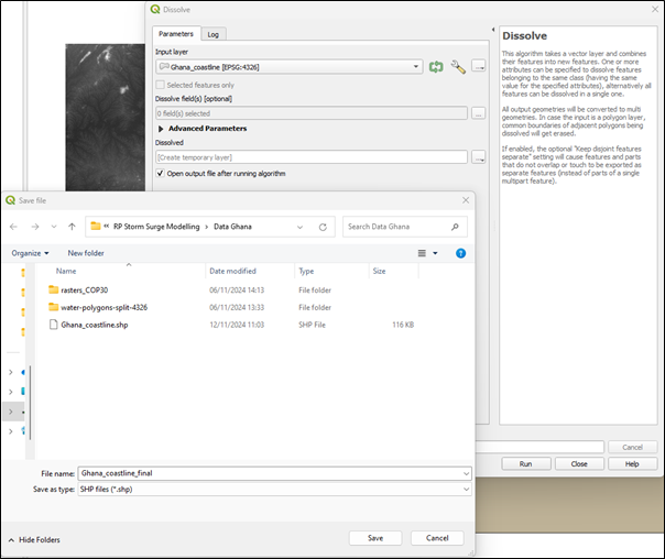
The clipped vector coastline layer is still divided into several tiles. To merge them into a single connected tile, search for 'Dissolve' in the Processing Toolbox. Fill in the parameters as shown in the screenshot (Fig. 13). Remember to save the layer in the respective folder, naming it for instance 'Ghana_coastline_final'. After selecting the folder, click 'Run' to create the final coastline.
You can remove the 'Ghana_coastline' layer to keep only the necessary layers in your QGIS project. The layer will now appear as shown in Figure 14.
3.2 DEM - Vertical and horizontal reference system adjustments
Note: If you aim to compare different digital elevation models, it is important to adjust both, the vertical and horizontal reference systems. The horizontal Coordinate Reference System can be adjusted using the 'Warp (Reproject)' tool, which can be found in the Processing Toolbox. For the vertical adjustment, a reference model is required.
The COP30 DEM has the vertical reference system EGM08. Since this is suitable for the planned storm surge modelling, no further vertical adjustment will be made to the DEM.
4. a) Processing with step-by-step procedure
4.1 Load data in QGIS
If you followed the preprocessing steps you already have all the necessary data in your QGIS project (the Copernicus 30 m DEM and the preprocessed shoreline layer, see Fig. 14). If you have your own datasets, please load a DEM and shoreline layer in your QGIS project.
4.2 Raster calculation
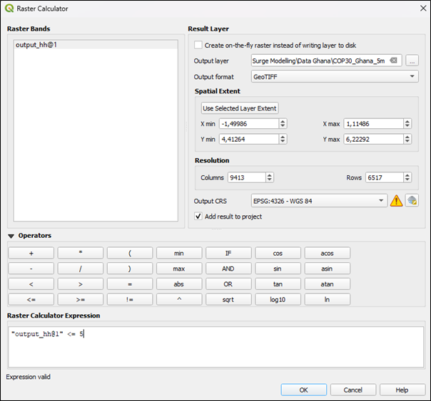
In this step, all elevation pixels below a certain elevation threshold will be detected. Open the Raster Calculator by selecting Raster > Raster Calculator (Fig. 15).
First, select your DEM layer and click on the ‘less or equal’ (<=) math operator to create a Raster Calculator Expression. Then set the threshold for the flood level you would like to simulate. In this sample case, a value of 5m has been set. In the equation you can also adjust the m to any height you like. Save your layer under ‘Output layer’ (here named: COP30_Ghana_5m) and set the ‘output format’ to GeoTIFF (Fig. 15).
The result is a binary raster layer that classifies all potentially flooded areas with a value of 1 and non-flooded areas with a value of 0 (Fig. 16). The results of step 4.2 are depicted in Fig. 16, where all pixels at or below 5m are represented in white, and pixels above 5m are represented in black with a value of 0.
4.3 Define NoData value
In this step, all non-flooded areas in the classification mask will be set to NoData using the ‘Translate (Convert Format)’ tool. The tool is accessed via Raster > Conversion > Translate (Convert Format). Set the ‘Input layer’ to the 5m raster layer, produced in section 4.2 and save the new layer under ‘Converted’ (here named: COP30_Ghana_5m_0_set_nodata). The NoData value has to be assigned to 0 (Fig. 17). Click Run.
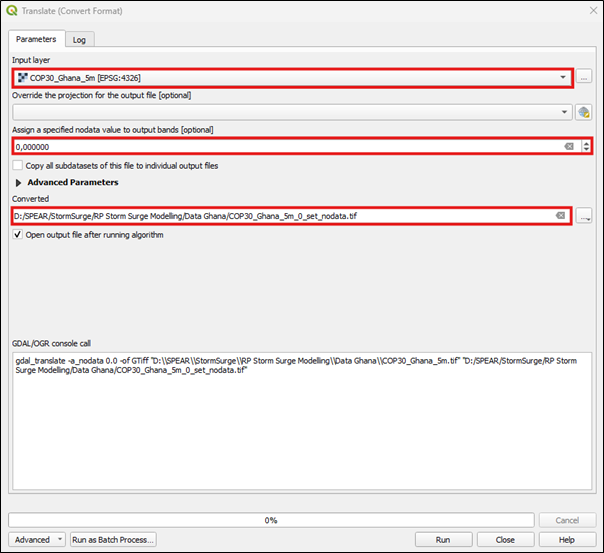
While the black area previously had a value of 0, it no longer has any value. The white area still retains the value of 1, indicating the flooded area and other water bodies.
4.4 Polygonize
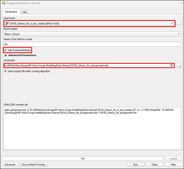
In this step the flooded area (area with the value 1) is going to be converted to a vector file using the Polygonize tool. Open the tool through Raster > Conversion > Polygonize (Raster to Vector) and set the input file (here: COP30_Ghana_5m_0_set_nodata). Save the polygonized layer under ‘Vectorized’ (here: COP30_Ghana_5m_polygonized). Tick the ‘Use 8-connectedness’ box (Fig. 18). Click ‘Run’.
4.5 Filter inland water patches
In this step, inland water patches that meet the elevation threshold (<= 5m) but are not connected to the ocean are filtered out. The connectivity between the ocean shoreline and the inland flooded areas is used to reduce the overestimation of flooded areas.
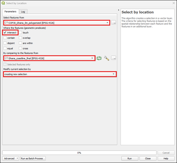
To identify only the flooded areas connected to the shoreline, the polygonized potential flood extent must intersect with the shoreline vector layer. This can be done using the 'Select by Location' tool, which is located under Vector > Research Tools > Select by Location.
Select the polygonized layer from the previous step as the 'Select features from' option. Tick the 'Intersect' box under the geometric predicate. For 'By comparing to the features from,' select the preprocessed coastline layer (from Step 3, here named 'Ghana_coastline_final'). Click 'Run' to proceed (Fig. 19).
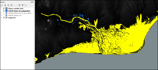
Note that you have now only created a selection of the polygonized layer (here: COP30_Ghana_5m_polygonized). The selected areas are highlighted in bright yellow in your QGIS project. Figure 20 shows an example, where the water patches connected to the shoreline are displayed in yellow, and the water patches that have not been selected (due to no direct connection to the shoreline) are shown in blue.
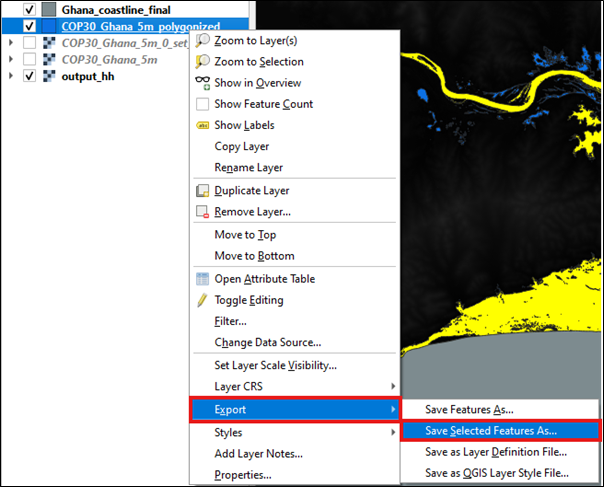
For saving the selected features in a separate layer, right-click on the polygonized layer then select Export > Save Selected Feature As (Fig. 21).
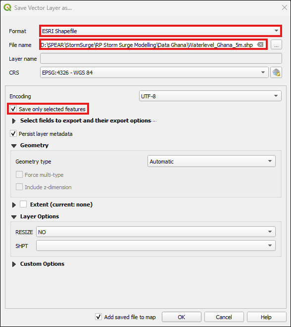
Change the format to ESRI shapefile and select a folder to save your 5m flood extent layer (here: Waterlevel_Ghana_5m): Make sure that the box ‘Save only selected features’ is selected. Click OK to save the new layer (Fig. 22).
You now successfully created the flood extent layer for a 5m flood height event. You can now proceed to step 5 and create a map with your layers. If you wish to create flood extent layers for different heights, you can repeat the steps 1 to 4 and adjust the water level height in step 4.2.
4. b) Processing with QGIS Model
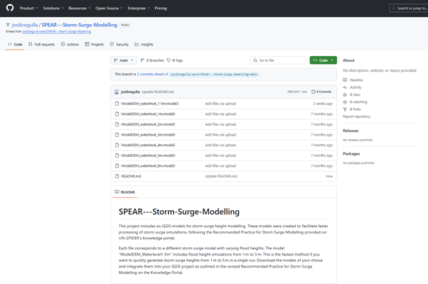
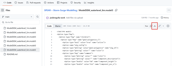
Another way to fulfill the steps (Processing 4.1 to 4.5) is by using the QGIS model provided at the following link (https://github.com/josibregulla/SPEAR---Storm-Surge-Modelling). In this GitHub project, you will find models that simulate surge heights ranging from 1 to 6 meters (Fig. 23). The 1-meter model includes the creation of a hillshade, which can serve as a visual enhancement for the final map. Download the models of your choice by clicking on the model and then on the download button on the top right (Fig. 24).
We begin again with step 4.1, 'Load data in QGIS', ensuring that both the DEM and coastline are loaded. Next, load the QGIS model (which you downloaded in the previous step) by clicking on Processing > Model Designer. The Model Designer will open. To load the downloaded model from GitHub, click Model > Open Model. Navigate to the model file (here: ModelDEM_waterlevel_5m), which you downloaded from GitHub, and open the model. Your screen should then display the following (Fig. 25):
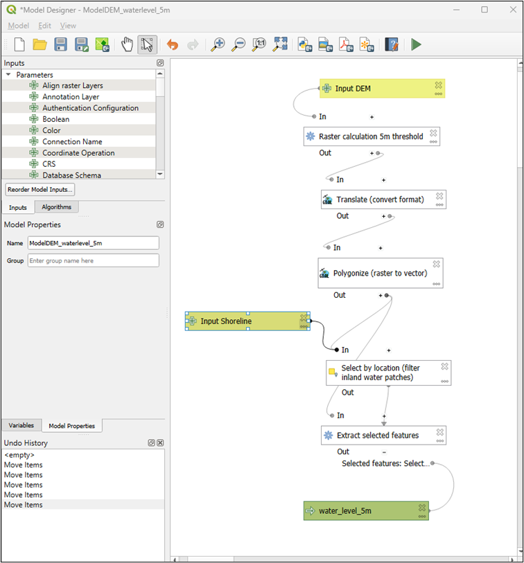
On the right side, you will see the QGIS model, which will automatically carry out steps 4.1 to 4.5. This approach offers the advantage of faster processing, particularly when assessing multiple areas worldwide and different storm surge heights.
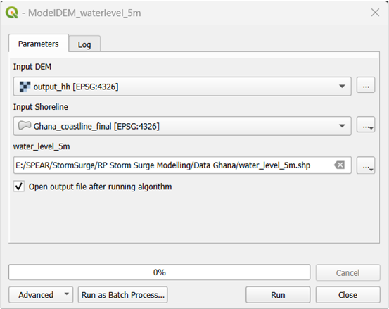
Click the green 'Play' button. Select the DEM, the preprocessed coastline, and save the layer. (Note: If you don't select a folder to save the layer in this step, a temporary layer will be created, automatically named 'water_level_5m') (Fig. 26).
Click ‘Run’. After a few seconds, you should get the following result (colors may differ; Fig. 27).
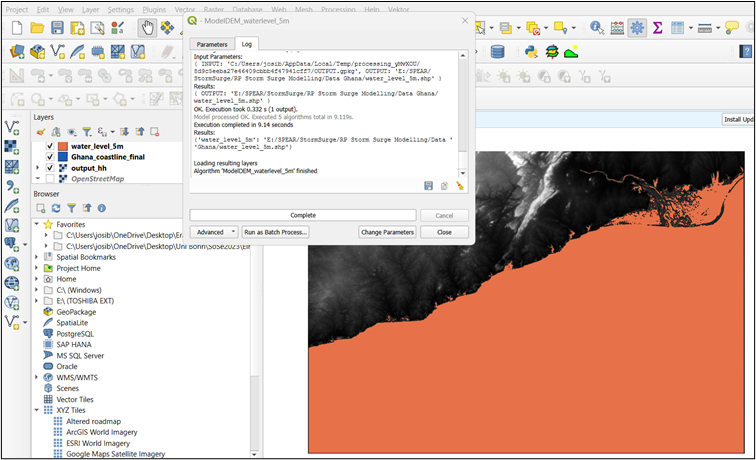
You have now created a flood height layer (here displayed in orange; adjust to the color of your choice in the next step) and can proceed to step 5 to create a thematic map.
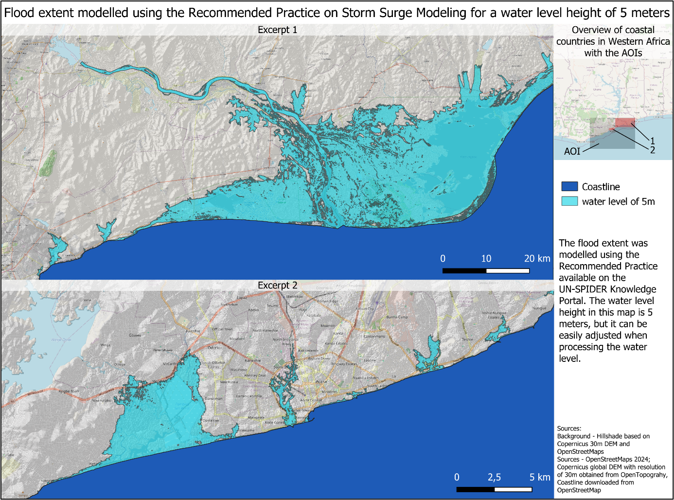
5. Create a map
The processed layers, including the final layer from Step 4a) or 4b), the coastline layer, and the DEM, can now be used to create a map showing the extent of the flood. You may add additional base maps or create hillshades to enhance the visualization. An example map is provided in Figure 28.