This Recommended Practice explains how to conduct a supervised land cover classification followed by a change detection analysis. In this application, the method is applied for an area of rainforest in the Amazon to detect forest loss. The data requirements for this analysis are at least two cloudless satellite images of the same area at a different point of time. This data will be used in order to uncover the land cover change between the two images. For this analysis, 2 Landsat 8 images of the area south of Santarém, Pará in Brazil from 14-08-2019 and 24-07-2019 were used.
Step 4: Supervised Classification
- 4.1: Create training input
- 4.2: Create classes
- 4.3: Change Band Rendering
- 4.4: Create ROIs
- 4.5: Assess ROIs
- 4.6: Run classification
Step 5: Change Detection
Step 6: Results
The data requirements for this analysis are at least two cloudless satellite images of the same area at a different point of time. This data will be used in order to uncover the land cover change between the two images.
Important: there should be no cloud coverage on the image, as this will distort the classification. This would greatly reduce the quality of the results.
There are various satellites which can be used as a data source. Via the Copernicus Data Space Ecosystem (https://dataspace.copernicus.eu/), satellite imagery of the European Union Copernicus programme, such as Sentinel 2 satellite data, can be accessed. Sentinel-2 provides high resolution data at a 10m resolution. Note that registration is required. The advantage of using Sentinel 2 satellite data is their high resolution, which makes classification more precise. The disadvantage is that data is only available from June 2015 onwards, meaning that it cannot be used for earlier change detection. Furthermore, EO Browser contains the full archive of the Landsat missions.
The Landsat mission provides satellite data for earlier dates: Landsat 4 since 1982 (until 2001), Landsat 7 since 1999 and Landsat 8 since February 2013. The disadvantage compared to Sentinel is that the resolution is lower, meaning that the classification is slightly less precise; Landsat 4 and 7 have a resolution of 30m and Landsat 8 has a resolution of 15m. Note that Landsat 7 suffers from a line corrector failure since 31 May 2003, resulting in black strips through all the images after this date.
Figure 1: Copernicus Data Space Ecosystem
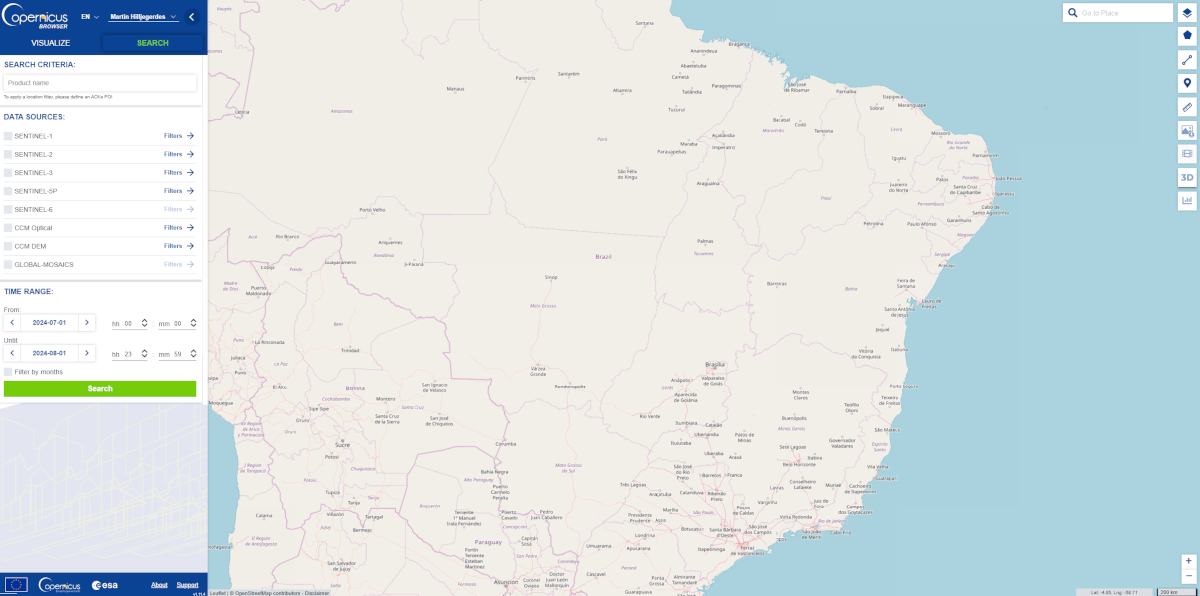
Figure 2: Copernicus Data Space Ecosystem Search Panel
Search data by ticking the boxes of the Sentinel 2 and choosing MSI -> L2A as the Product Type. Sentinel 2 Multi-Spectral Instrument L2A is the atmospherically corrected version of the data. This is compared to S2MSI L1C in which differences in water moisture and other atmospheric conditions between the before and after images may alter the change detection.
Next, use the slider below to specify the Cloud Cover %. As mentioned, the lower the amount of cloud cover is the better the results will be. You can visually inspect an image to ensure your area of interest is clear.
Then apply the appropriate time range for the image Sensing Period, create an Area of Interest (tool on the top right) and click search.
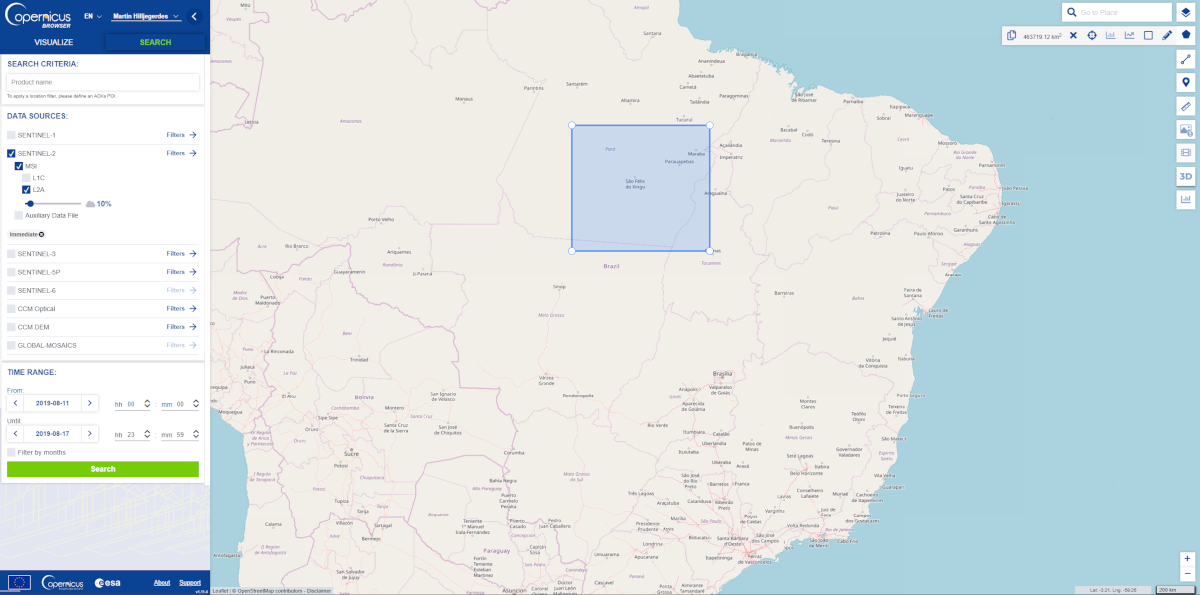
Figure 3a: Copernicus Data Space Ecosystem Search Panel
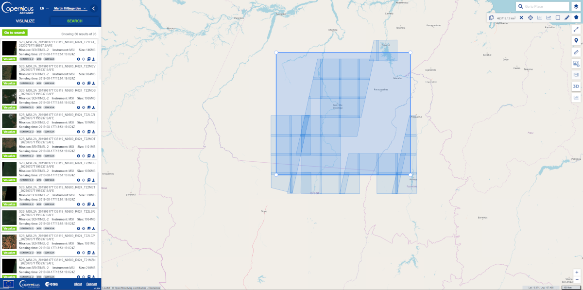
Figure 3b: Copernicus Data Space Ecosystem Search Panel Results
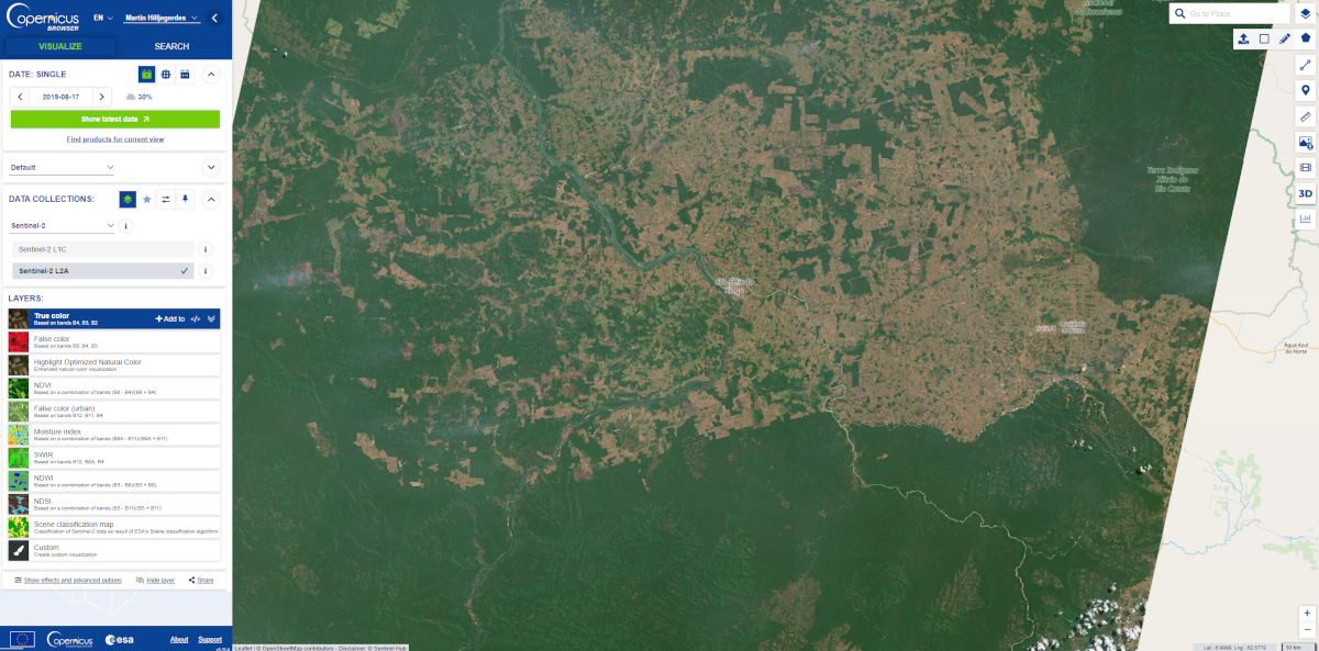
Figure 3c: Copernicus Data Space Ecosystem Result Visualization
Results will pop up in the results window. Each result shows a small preview, the data and date. You may click the "i" symbol next to an individual result; this will give more information about each of the data files. You can also click the "Visualize" button to inspect an individual scene in more detail.
For the classification and change detection, date and cloud cover are most relevant. Make sure that, even for an image with low cloud cover, the area that you want to analyse contains no clouds.
For this step it is important for the user to be logged in to the Data Space Ecosystem. After choosing the preferred image, click the download button.
Complete Step 1 for both a before and after image of your area of interest.
Alternatively, to access Landsat datasets you can use USGS Earth Explorer (https://earthexplorer.usgs.gov/).
For this analysis, 2 Landsat 8 images of the area south of Santarém, Pará in Brazil from 14-08-2019 and 24-07-2019 were used.
QGIS is an Open Source Geographic Information System (GIS) licensed under the GNU General Public License. QGIS is an official project of the Open Source Geospatial Foundation (OSGeo). It runs on Linux, Unix, Mac OSX, Windows and Android and supports numerous vector, raster, and database formats and functionalities (QGIS). There are various versions of QGIS available. For this analysis, it is advised to download the latest stable version. This practice used QGIS 3.2 Bonn for the analysis.
Once QGIS is downloaded, navigate to Plugins > Manage and Install Plugins.
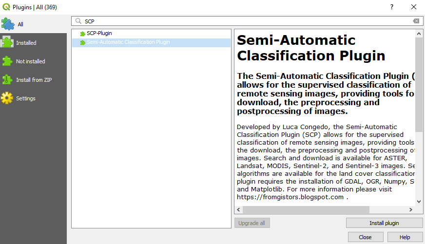
Figure 4: QGIS Install Plugin Window
In the screen, search for Semi-Automatic Classification Plugin and click Install plugin. Once installed, a new Panel should pop up in the main QGIS window: The SCP Dock. If this does not happen automatically, navigate to View > Panels and toggle SCP Dock. The SCP Dock is displayed in the image below.
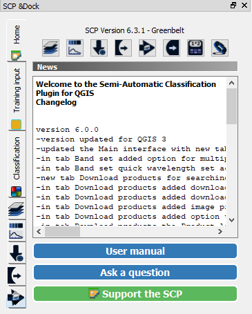
Figure 5: SCP Dock
Additionally, the SCP Working Toolbar and SCP Edit Toolbar should appear. These can be toggled by navigating to View > toolbars. The SCP toolbar is displayed in the image below.

Figure 6: SCP Toolbar
Make sure all the assets are toggled as they are needed for the analysis.
Now the data has been downloaded and the software is ready for use, the data can be imported into QGIS. Do so by navigating to your first set of satellite images in the browser panel and drag all the bands that are numbered into the Layers panel: This means that bands such as a True color band are excluded. The number of bands can differ per Satellite. For Landsat 8, there are 9 bands as depicted in the image below.
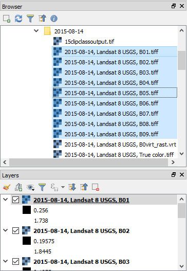
Figure 7: QGIS Browser Panel
The directory in which the data is saved must be loaded into the SCP plugin. Do so by navigating to SCP (in the main toolbar) > Preprocessing > select the satellite of which the data is from. In this case, it is Landsat.
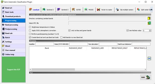
Figure 8: SCP Plugin
Click on  and navigate to the directory which contains the satellite bands. Select the folder and close the preprocessing window by clicking on the X in the top right corner. Important: close it without running it.
The next step is to create one layer of all the bands combined, called a band set. Do so by navigating to SCP > Band set.
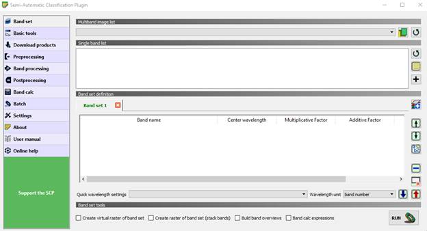
Figure 9: SCP Bandset page
Click  near the Single band list in order to show the bands which are contained in the directory loaded in the previous step.
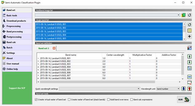
Figure 10: SCP Plugin Banset Window with the Single Band List loaded
Select all the numbered bands and click the  icon to add them to the band set definition. For Sentinel 2 this includes band 8A but for both Landsat and Sentinel make sure not to include the True Color Image (TCI). Toggle ‘Create virtual raster of band set’ and click run. Save the output in a designated folder: It is advised to save the output in the same folder as the satellite band.
Make sure that the raw bands and the virtual raster are loaded as layers. Click the  in the QGIS main toolbar. When clicking on any pixel of the virtual raster, reflectance values for each band will appear in the identify results panel as shown below.
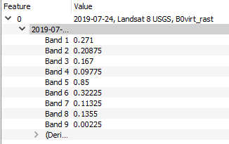
Figure 11: Pixel information for each band
These values change depending on what type of land cover is clicked and stay relatively constant for the same types of land cover. The classification will be based on the differences and similarities of these value combinations.
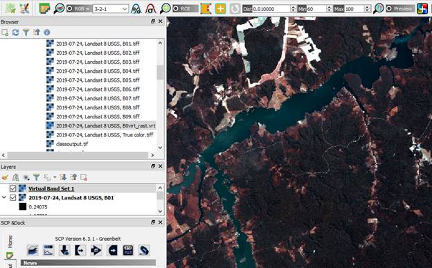
Figure 12: Area image before changing band rendering
After changing the band rendering from 3-2-1 to 5-2-1, it is much easier to distinguish between water and forest as is visualized in the image depicted below.
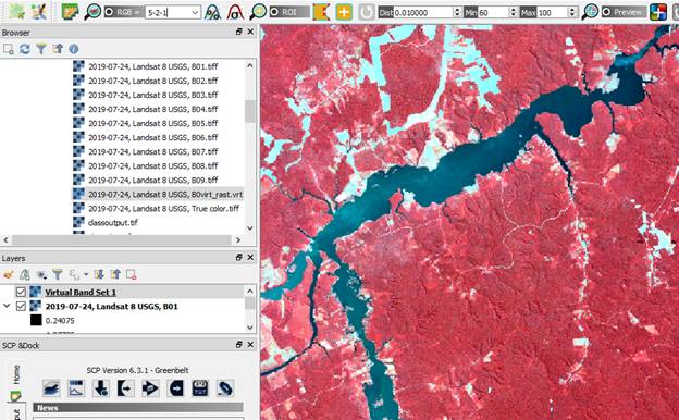
Figure 13: Area image after changing band rendering
In order to apply this change, change the band numbers in the SCP Toolbar  to
to  . Alternatively, right click on the virtual band set layer and navigate to Properties > Symbology
Step 4: Supervised Classification
In order for QGIS to run a classification, it will need to know what specific areas of the image – and what underlying values – belong to which class. Classification is a remote sensing technique which categorizes the pixels in the image into classes based on the ground cover. This is done by comparing the reflection values of different spectral bands in different areas. In supervised classification, the user determines sample classes on which the classification is based while for unsupervised classification the result is solely the outcome computer processing. In this case supervised classification is done. Therefore, training inputs will have to be established.
Create a new training input by navigating to training input in the SCP Dock and clicking on the  icon. Name and save the file in the same folder as the satellite data.
It is up to the user to determine which and how many classes there will be. However, for change detection, the number of classes should be kept relatively small. The more classes, the more complex the change matrix and future analyses will be. In this Recommended Practice the goal of the analysis is to find out how much forest has been lost between 2015 and 2019. The classes that are used in this are depicted in the image below. To create classes, navigate to the Macroclass list under Training Input in the SCP Dock. Add classes by clicking the  icon and change the name by clicking inside the MC info cell. Make sure that each class has a unique MC ID value like in the image below.
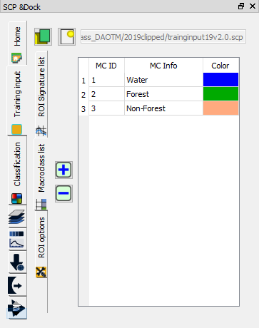
Figure 12: SCP Dock Macroclass list
Band rendering lets you change the visualization of the map. This is a useful tool to make land cover classes appear more distinct from each other. For example, water in the image below is difficult to identify, as the color of rainforest is fairly similar.
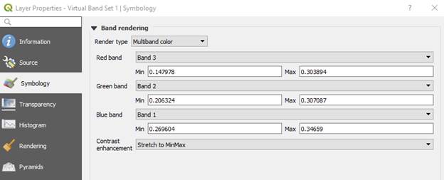
Figure 13: Layer Properties, Symbology
In this window, the Bands can be changed via the drop-down menu for each color. The band rendering can be changed at any moment throughout the classification process.
Once the classes have been created, go to the ROI signature list where you can start adding ROIs.
There are two types of ROIs that can be created. One is by drawing a polygon yourself of an area which you can clearly see belongs to a specific class. Do so by clicking the  icon which can be found on the SCP toolbar. Now draw a polygon on the map. By right clicking you can finish the polygon.
Next, make sure that the polygon is assigned to the correct class by changing the MC ID. In the image below, the polygon that will be saved will be assigned to the water class (MC ID 1).
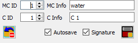
Figure 14: ROI Polygon class and MC ID info
Now click the  icon in the SCP Dock to save the polygon.
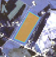
Figure 15: ROI Polygon
A second option is to add a group of pixels as an ROI by clicking on  . Now click on a pixel on the map of the specific class. QGIS will automatically select the surrounding pixels which have the same or similar reflection values. Saving works the same as for drawing the polygons.
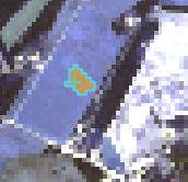
Figure 16: ROI by similar pixels
Create at least 10 ROIs for each class. The more the better, but precision is important. If pixels are assigned to the wrong class, a poor classification output is likely.
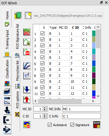
Figure 17: List of ROIs in SCP Dock
Once the ROIs are created, they can be visualized in a spectral signatures plot by highlighting the ROIs and clicking on  . This is a handy tool to assess the quality of the classification.
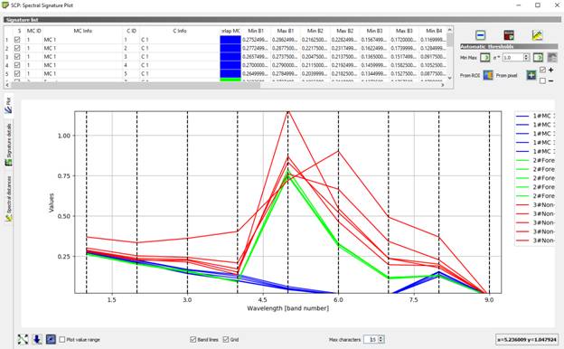
Figure 18: SCP: Spectral Signature Plot
The plot shows the values for a ROI for each wavelength. The dotted lines represent each band of the Landsat image. As can be seen in this graph, the water (blue) and forest (green) all have very consistent values within their class, while the third class, non-forested, is much more heterogeneous. This can be explained by the large variety of land cover falling under this class, ranging from agriculture to buildings. However, classes in which ROIs have very similar values are preferred as this increases the precision of the classification.
A second way of assessing the ROIs is doing a preview of the classification. Do so by clicking the  icon on the SCP toolbar and clicking an area on the map. This area will now be classified, so the precision of the output can be assessed. The image below displays an example of a preview.
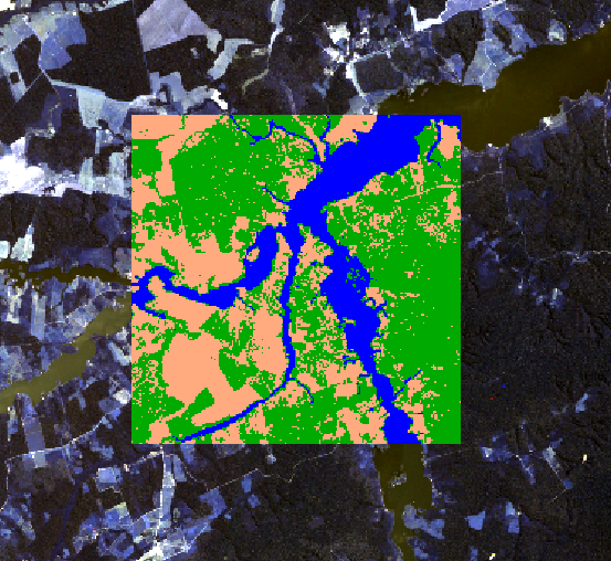
Figure 19: Preview of classification
content with the quality of the ROIs, the classification can be run for the entire image. On the SCP dock navigate to the classification window.
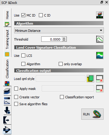
Figure 20: SCP Dock
Make sure that MC ID is ticked, and that the algorithm runs Minimum Distance. Run the classification. This will create a layer for the entire area which looks similar to the preview and the image below. The coloring can be changed in the properties window of the layer (right click on layer > Properties > Symbology).
Note: In this Recommended Practice, the Minimum Distance algorithm was run as this gave better results. However, it might be possible that in a different instance the Maximum Likelihood algorithm has better results. Hence, it is advisable to run both algorithms and choose the one with the best results.
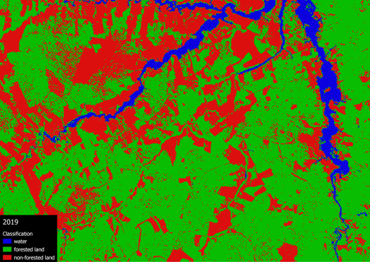
Figure 21: Ground cover classification
Save the layer as a GeoTiff file by right clicking on it and navigating to Export > Save As.
Repeat Step 3 and Step 4 for the second image. Make sure that this image is from the same satellite, of the same region but at a different point in time. Additionally, make sure your recreate your Macroclass list identically, with the same names, numbers and MC IDs for each class as done for the first image. Create new ROIs for your second image and run the classification again.
There are now two classification layers. Make sure both are loaded into the QGIS layers panel. Navigate to SCP > Postprocessing > Land Cover Change.
Load the oldest classification layer as reference classification and the latest classification as new classification. Make sure the “report unchanged pixels” box is ticked, as this provides valuable information for the interpretation. Then click Run.
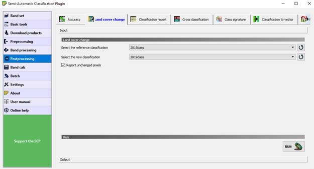
Figure 22: SCP Plugin Land Cover Change Tab
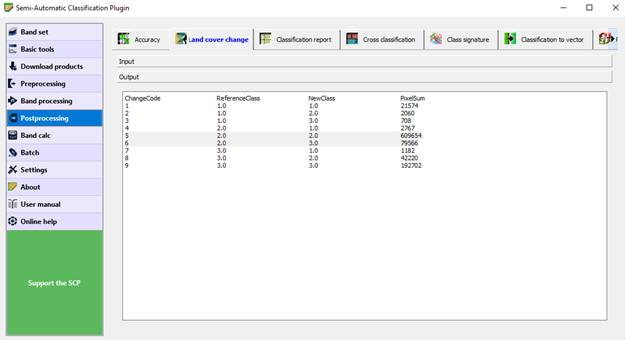
Figure 23: SCP Land Cover Change Outputs
The output window displays a table which shows how many pixels have changed to a different class. In this example, changecode 6 displays how many pixels changed from forested (ReferenceClass 2.0) to non-forested (Referenceclass 3.0) which represents deforestation.
QGIS also creates a layer for the change detection analysis. For this analysis, we mainly want to focus on forested land becoming non-forested land. Hence, we want to visualize the pixels that have changed from class 2 to class 3. Do so by going to properties > symbology. Change Render type to Paletted/Unique values and click on classify.
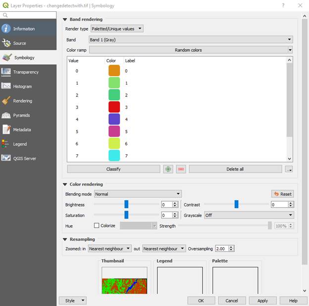
Figure 24: Layer Properties, Symbology
Because we are only interested in Changecode 6, change all other colors to black and choose a preferred color for 6. Click on apply and OK.
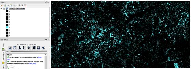
Figure 25: Land Cover Change Output Map
This gives an output where only the pixels are highlighted which were deforested. The layer can be saved and exported or further processed into a map in QGIS.