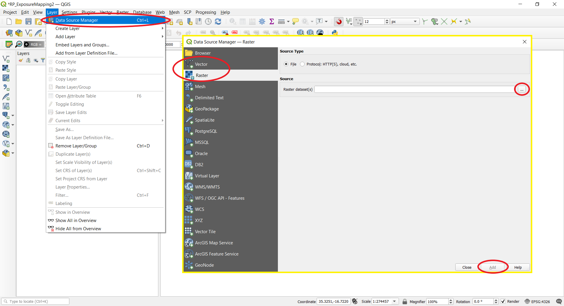
1.1 Load the flood mask and administrative boundary shapefile into QGIS. Go to Layer --> Data Source Manager, browse the data in their respective formats (raster or vector) on the left panel --> Add. After importing the data, make sure they have the same projection (WGS84) by checking in the Properties --> Source of each layer.
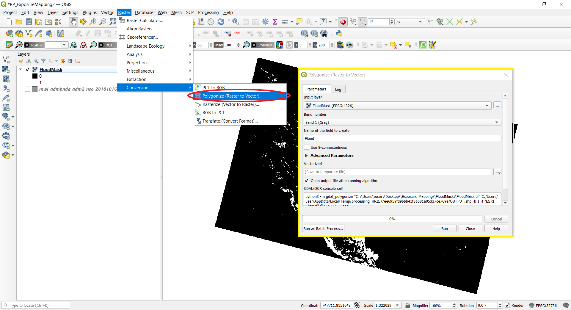
1.2 If the flood mask is a raster file (.tif), convert it to a vector file (.shp), skip this step if the flood mask is already a vector file. Open Raster --> Conversion --> Polygonize, select the flood mask raster as the input, and name the field to create as "Flood", click Run.
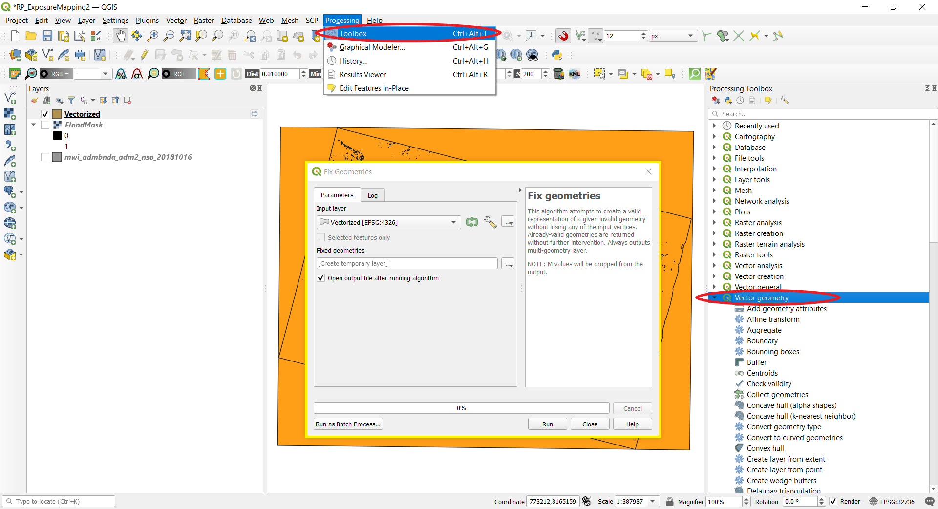
1.3 The new vectorized layer will appear on the map. To ensure the layer can be further processed without errors due to invalid polygons from conversion, open Processing --> Toolbox, then in the Processing Toolbox, go to Vector geometry --> Fix geometries (or simply search for Fix geometries). In the Fix geometries window, select the Vectorized layer as the input and click Run.
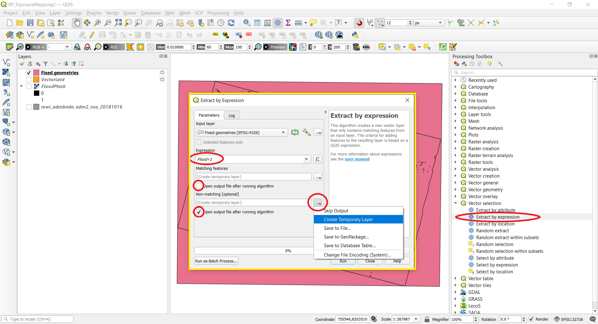
1.4 To have the flood mask layer without the background polygons (no water), go to the Processing Toolbox --> Vector selection --> Extract by expression. Set the Fixed geometries layer as the input layer. Put "Flood<1" in the expression box because the vectorized flood mask stores the data in its attributes indicating 1 as flood and all the numbers smaller than 1 as not flooded. As we want to extract the flooded areas which is the data that is non-matching to the expression, unselect the checkbox under Matching features, change the output setting for Non-matching features to [Create temporary layer] and select the checkbox. Click Run.
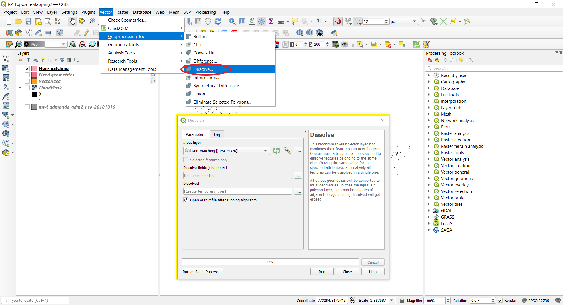
1.5 Merge all the remaining polygons into one single polygon that indicates the flood area. Open Vector --> Geoprocessing Tools --> Dissolve, select the extracted layer as the Input layer --> Run.
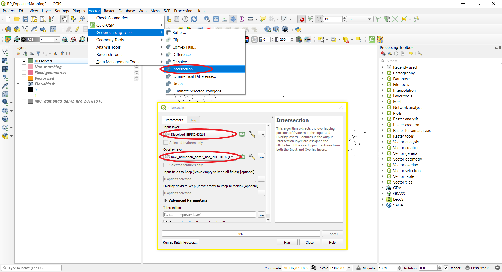
1.6 Using the Administrative Boundary layer, cut out the flooded areas that is not within Malawi. Go to Vector --> Geoprocessing Tools --> Intersection. Select the dissolved layer as the input layer, and the administrative boundary layer as the overlay layer --> Run. By overlaying a district-level boundary layer, the flood polygon will split into its respective districts, this can help with analysis purposes. For this case, the polygon is split-up into three as it intersects with three different districts.
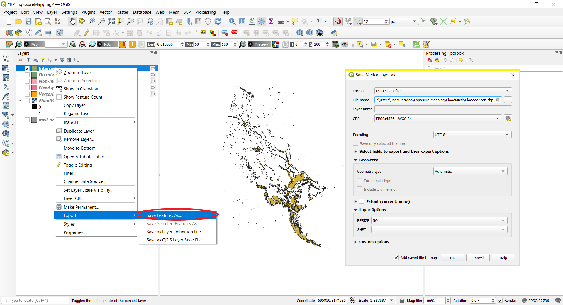
1.7 As the processed layers in the previous steps are temporary, save the prepared Intersected flood mask layer by right clicking on the layer --> Export --> Save Features As. Select the desired format and destination of the file, make sure the coordinate reference system (CRS) is the same with the other layers (WGS 84) and the box next to "Add saved file to map" is checked.
2.1 Load the population data, go to Layer --> Data Source Manager --> Raster.
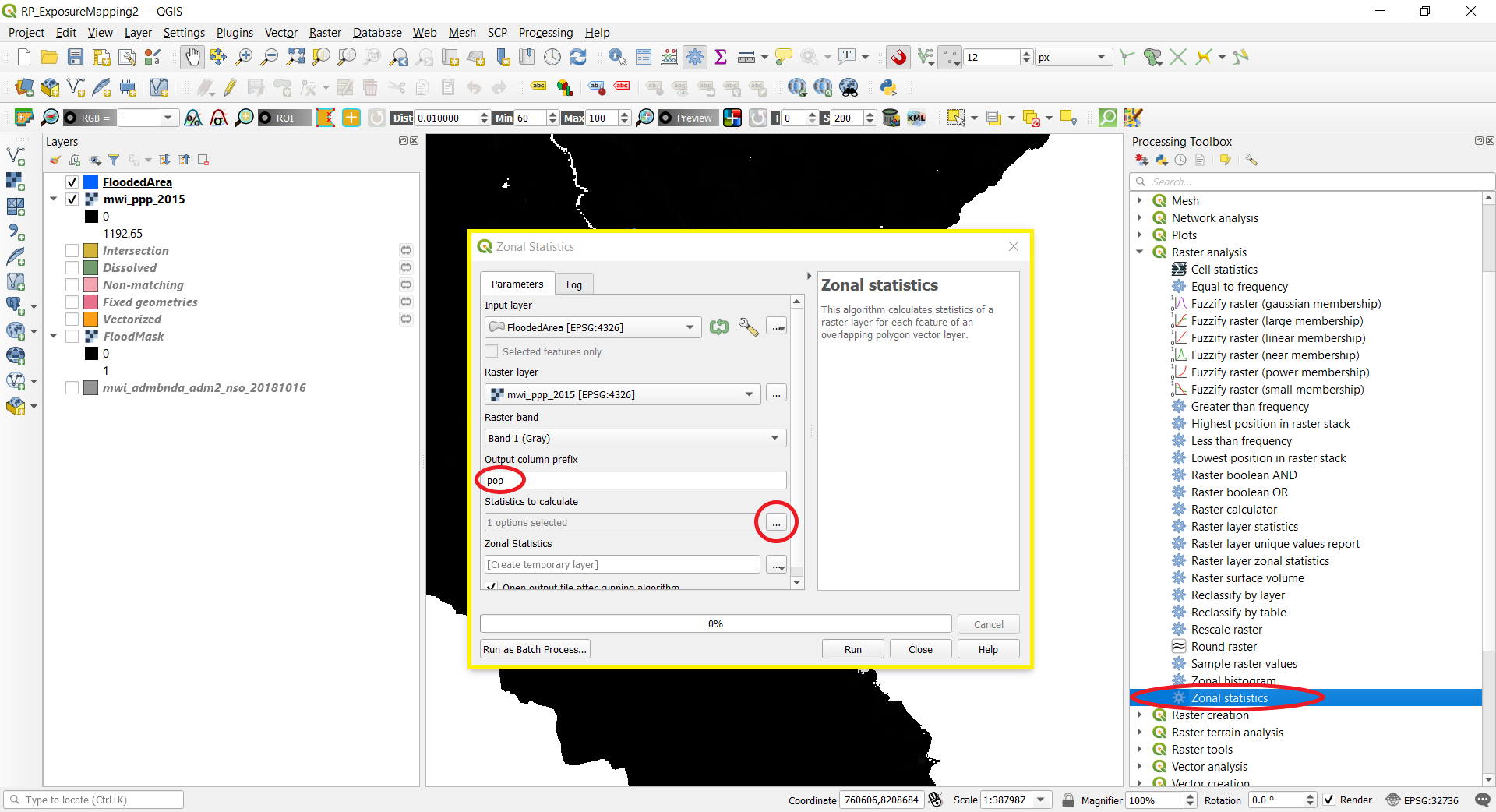
2.2 The Zonal statistics function can be used to receive the population data solely for the flooded area. Go to Processing Toolbox --> Raster analysis --> Zonal statistics (Note: make sure it is "Zonal statistics" not "Raster layer zonal statistics"). Selected the processed flood mask vector as the Input layer, and the population raster as the Raster layer. Define an output column prefix ("pop" for population) and check Sum under Statistics to calculate. Click Run.
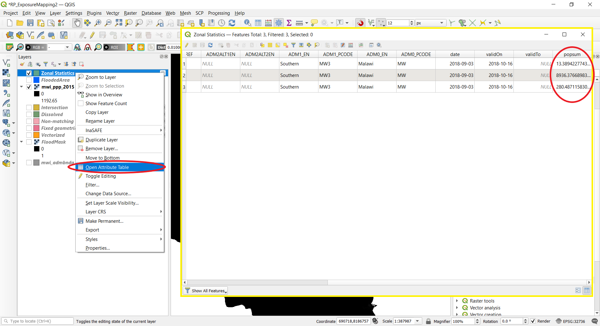
2.3 Look at the Attribute Table of the new Zonal Statistics layer by right clicking on the layer --> Open Attribute Table. The field "popsum" indicates the total population in each district that falls within in the area of interest (flooded area). Note that this number is affected by uncertainties.
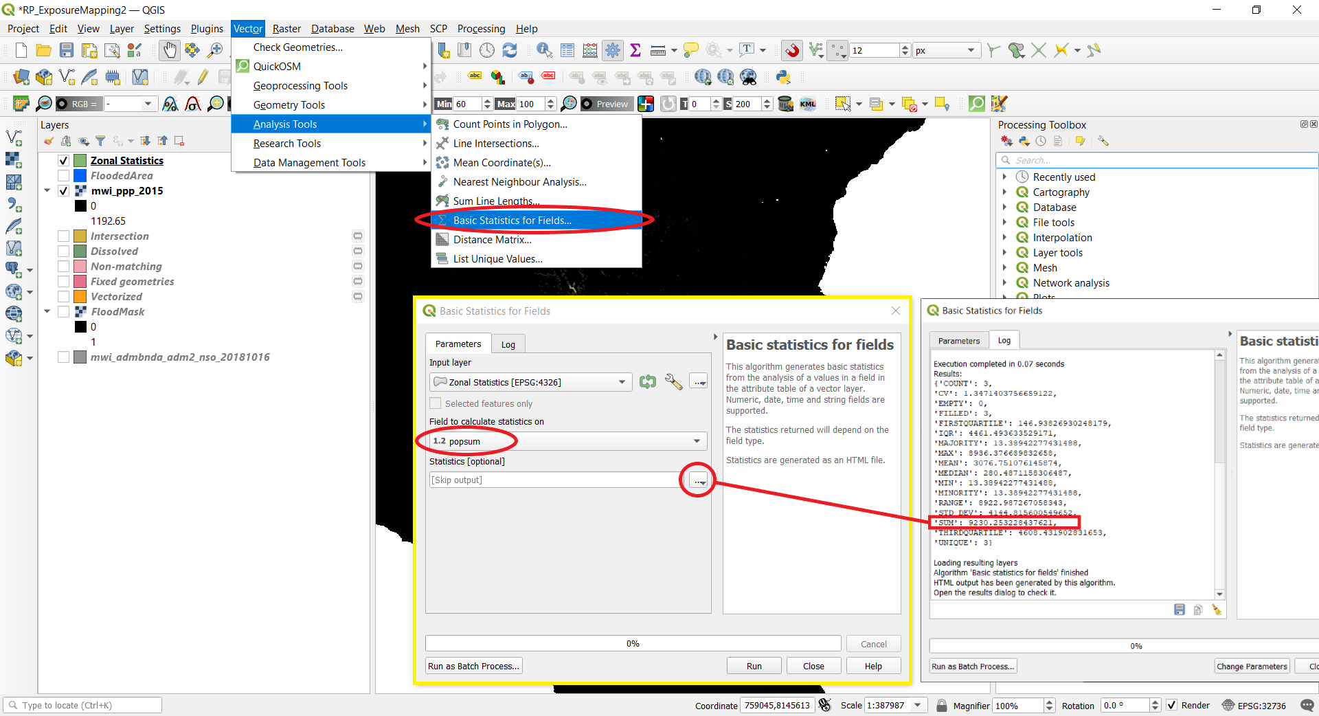
2.4 To get the total number of affected population, apart from manually calculating the number, this can also be done through QGIS tools. Go to Vector --> Analysis Tools --> Basic statistics for fields. Select the Zonal statistics layer as the Input layer, popsum as the Field to calculate statistics on, and skip output. Click Run, then in the same window under Results, you will find the statistics to the layer, and specifically Sum: 9230 as the total affected persons within the entire flooded area.
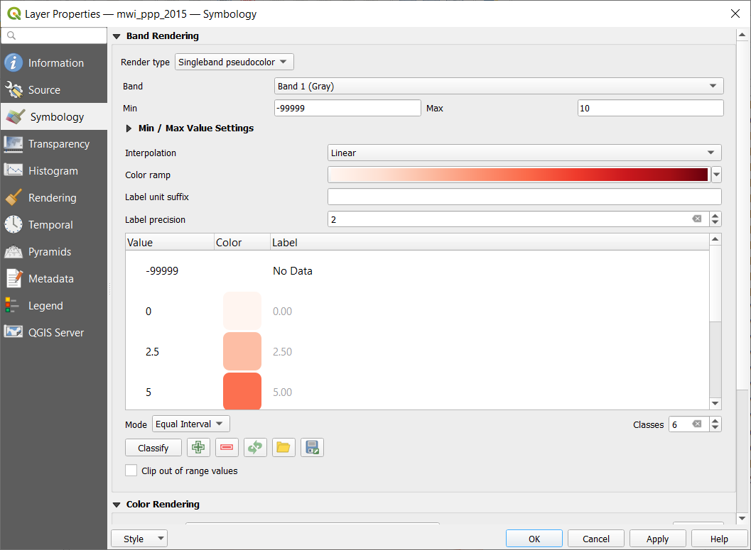
2.5 Change the style of the layers to better visualize the data (right click on the layer --> Properties --> Symbology). For example, change the flood mask to blue and lower its opacity so that it is half-transparent; change the population data Render type to Singleband pseudocolour, tinker the min/max and classifications, and choose a colour bar.
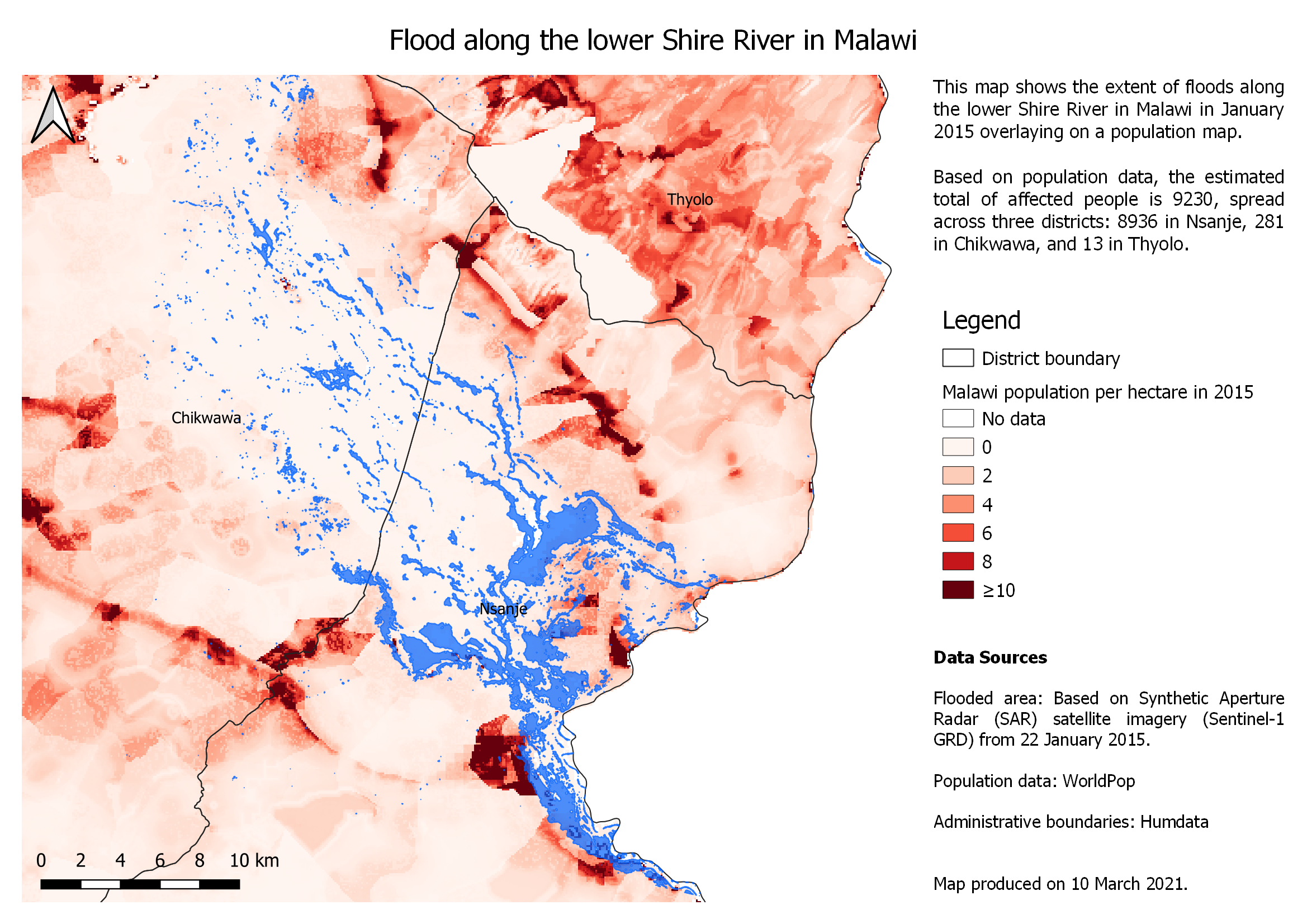
2.6 To create a map with simple description of the analysis, legend, scale bar, and north arrow, you can create a new print layout (Project --> New Print Layout). Below is an example of a final exposure map in the context of population.
3.1 Load the land cover data, go to Layer --> Data Source Manager --> Raster. Ensure the projection of the layer is in UTM, or else the area calculation in the next steps will not be in square meters.
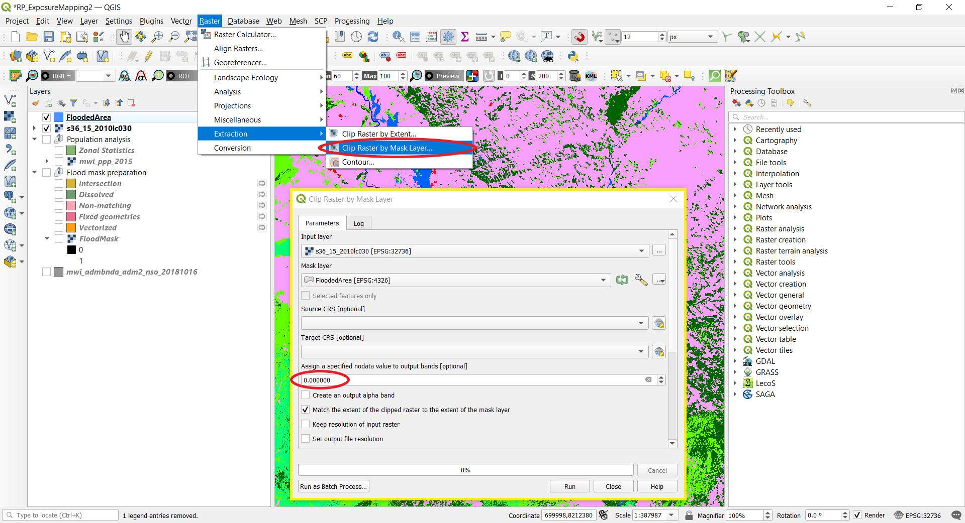
3.2 Clip the land cover raster to the extent of the flood mask. Open Raster --> Extraction --> Clip Raster by Mask Layer. Select the land cover raster as the Input layer, the flood mask vector as the Mask layer, and assign a specified nodata value to 0 --> Run.
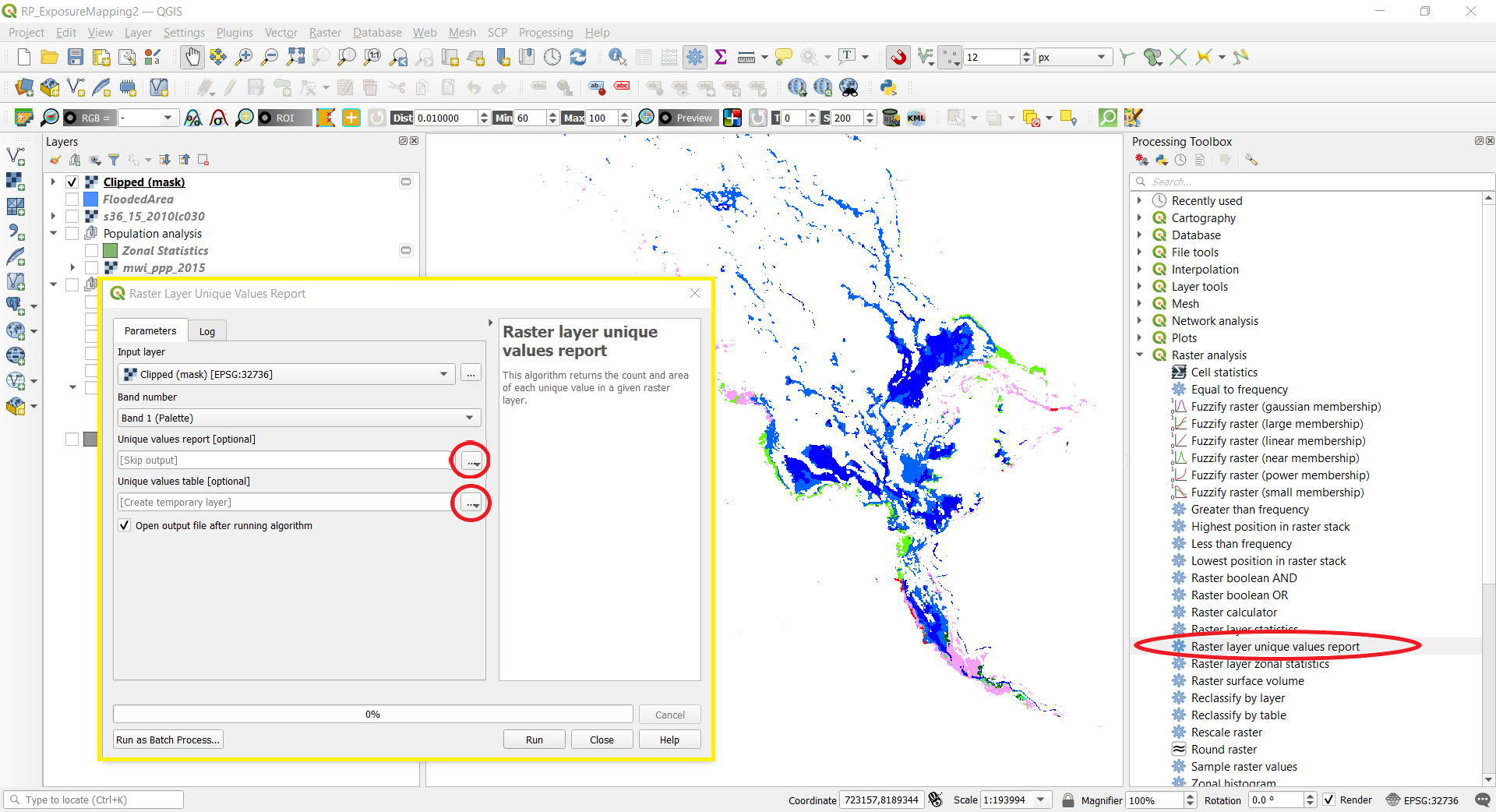
3.3 The clipped land cover raster will appear on the map, you might have to turn off or re-order the other layers to see it. To estimate the area and types of affected land cover, go to the Processing Toolbox --> Raster analysis --> Raster layer unique values report. Selected the clipped land cover layer as the Input layer, [Skip output] for Unique values report, and [Create temporary layer] for Unique values table --> Run.
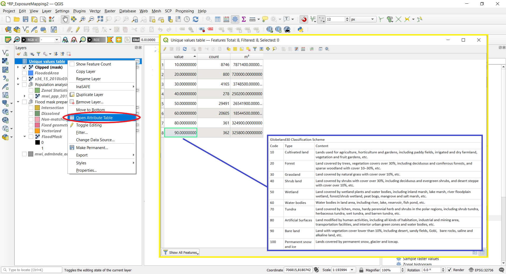
3.4 To view the calculated values of affected land cover, right click on the newly created Unique values table --> Open Attribute Table. The value field indicates the land cover type, the classification scheme (extracted in screenshot below) can be found in Section 3 of the Globeland30 Product Description, note that the classes are generalized. The count field indicates the number of pixels. The ㎡ field shows the calculated area in square meters, the number can be converted into hectare by dividing 10000 or to square kilometers by dividing 1000000.
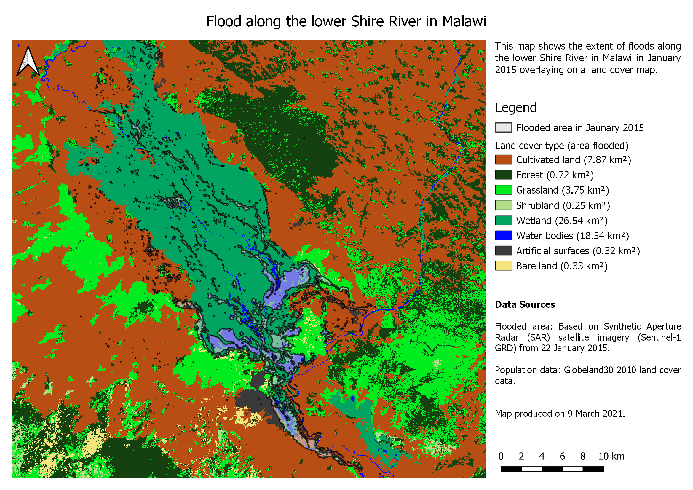
Therefore in our case, approximately 7871400 square meters of cultivated land (class 10) and 324900 square meters of artificial surfaces (class 80) were flooded.
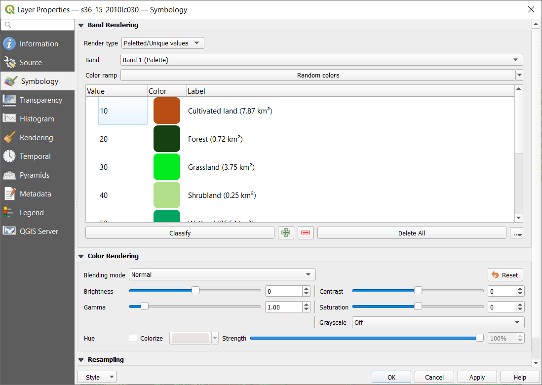
3.5 Change the style of the layers to better visualize the data (right click on the layer --> Properties --> Symbology). For example, change the land cover data Render type to Paletted/Unique values, click "Classify" to group the values, choose the appropriate colours and rename the labels.
3.6 To create a map with simple description of the analysis, legend, scale bar, and north arrow, you can create a new print layout (Project --> New Print Layout). Below is an example of a final exposure map in the context of land cover.