The step-by-step procedures below are for the free software "R'.
(Click here to access step-by-step instructions for ENVI version 4.8.
Click here to access step-by-step instructions for Envi 5.)
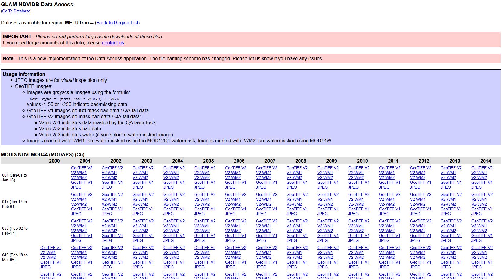
Two-weeks normalized Differenced Vegetation Index (NDVI) composits based on 250m MODIS data are freely available for download from the MODIS/NDVI Time Series Database from the Global Agriculture Monitoring (GLAM) Project provided via the website of Geographic Department of Maryland University. The Data Access App provides easy access to the data for different regions including Iran (cf. figure below). The Maximum Value Compositing (MVC) procedure was applied to derive the two-weeks composits. The resulting geotiff images are greyscale images using the formula ndvi_byte = (ndvi_raw * 200.0) + 50.0. Values below or equal 50 or larger than 250 indicate bad/missing data, which are masked in the geotiff V2 images. Additionally, two products come with a water mask: V2-WM1 using the MOD12Q1 watermask, and V2-WM2 using the MOD44W watermask; in both cases the value 253 indicates water.
Content
Step 1: Download MODIS 13Q1 data
Step 2: Download country shapefiles
Step 3: Reprojection of hdf into tif using MRT41
Step 4: Database and file naming
Step 1: Download MODIS 13Q1 data
Besides the GLAM NDVI data, the MODIS 13Q1 data set provides NDVI and EVI data at 250m resolution, which can be downloaded via the USGS Earthexplorer.
The MODIS13Q1 data has a certain way to name the single files. The name contains relevant information like acquisition date or acquisition tile.
Example for hdf files:
MOD13Q1.A2000049.h09v07.005.2006269133152.hdf
MOD13Q1 - Product Short Name
.A2000049 - Julian Date of Acquisition (A-YYYYDDD) --> 49th day of the year 2000
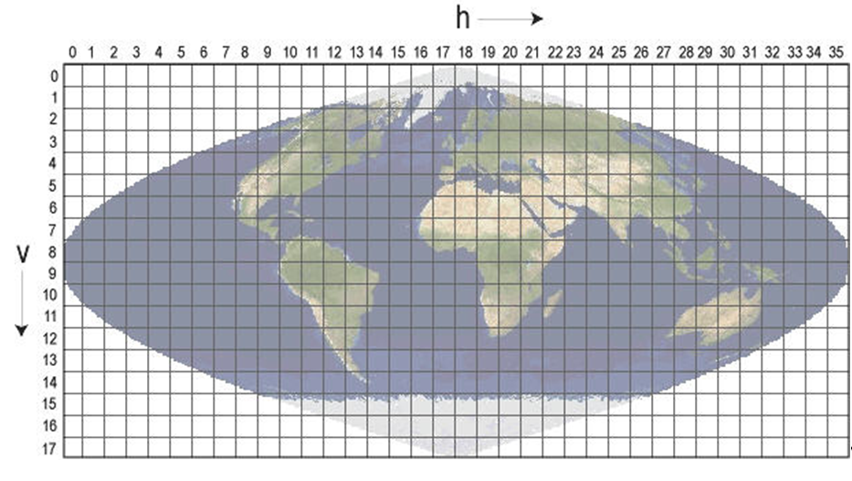
.h09v07 - Tile Identifier (horizontalXXverticalYY) --> see image below.
.005 - Collection Version
. 2006269133152 - Julian Date of Production (YYYYDDDHHMMSS)
.hdf - Data Format (HDF-EOS)
Example for tif files:
MOD13Q1.A2000049.250m_16_days_EVI.tif
MOD13Q1 - Product Short Name
.A2000049 - Julian Date of Acquisition (A-YYYYDDD) --> 49th day of the year 2000
.250m_ - spatial resolution
.16_days_EVI – temporal resolution à 16 days Maximum value composite
.tif - Data Format (GeoTiff)
Step 2: Download country shapefiles
Country shapefiles can be downloaded at http://www.gadm.org/country. Note: The boundaries and names of the shapefiles do not imply official endorsement or accesptance by the United Nations.
Step 3: Reprojection of hdf into tif using MRT41
If you have downloaded MODIS data in hdf format, you need to first convert them into tif files before using them in R software. These are the steps:
- Download and install Modis Reprojection Tool (MRT) (Download: https://lpdaac.usgs.gov/tools/modis_reprojection_tool)
- Open the MRT
- First, you have to create a Parameter File, which contains file names, types of input and output data files. Follow the steps below to create the parameter file.
- Select any one of the Input File to set parameters (File > Open Input File), which will be used lateron for the batch processing.
- Under "selected bands" select the bands you need and move the remaining bands to "available bands" by highlighting them and clicking on the arrow; in this case we are interested in NDVI and EVI.
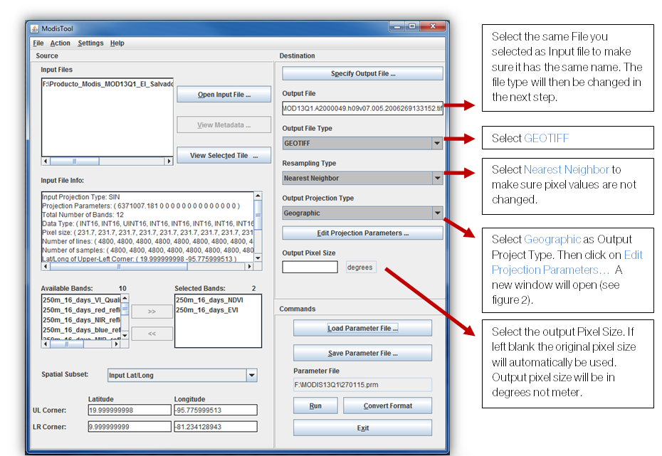
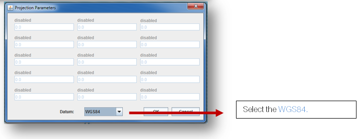
4. After inserting the parameters (cf. images above), save your Parameter File with Save Parameter File.
Note: Do not click on "run" nor on "convert format". The creation of parameter files for all input MODIS files as well as the conversion to tif will happen in the Command Prompt (cf. step 5).
5. Automated Batch Processing
In the following you will convert all the MODIS files (in hdf format) at once into tif format (batch processing). In summary these are the three steps for the batch processing:
- Gather all input files into one exclusive directory (containing nothing but MRT input)
- You will then create parameter files (.prm) for each input file in the input data directory with MRTBatch.jar. It also writes out a batch script that is later used to execute the processing jobs (MRTBatch.bat) (cf. below how to).
- Finally, you wil convert the hdf files into tiff files (cf. below how to).
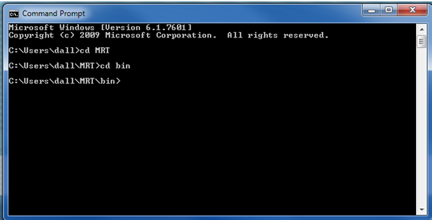
Click on Start > Search Programs and Files > Command Prompt
Using the Command Prompt, you then should navigate to the "MRT bin" directory, where the "MRTBatch.jar" file lays:
- cd folder - This command will move you to the folder that you specify. The folder must be in the directory you are currently in. For example: If you are currently at C:\Users\username\ and you enter cd desktop you will be taken to C:\Users\username\Desktop\
- dir - This command will list all of the folders and files in the directory you are currently at (this step is optional).
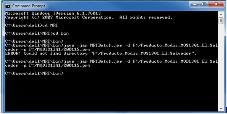
Type the following command to initiate parameter file and batch script generation (place all fields in one line; i.e., do not break this statement into multiple lines).
Note: the italic words have to be replaced by your actual directory or file name (cf. explanation below).
java –jar MRTBatch.jar –d input_directory –p parameter_directory\input_parameter_file –o parameter_directory
where
input_file_directory is the directory in which all input files are placed (e.g.,
C:\Project\InputFiles);
parameter_directory is the directory where the parameter file - created using the graphical user interface (GUI) of the MODIS Tool - was saved (-p) and to which the parameter files built by this application will be written (-o); Note that the –o parameter_directory is optional. Users can omit it from the command line, which will result in a prm directory containing the new parameter files being built in the input_file_directory instead.
input_parameter_file is the parameter file that was saved from the graphical user interface (GUI) of the MODIS Tool (e.g., mrtauto_test.prm).
Hit the enter key on your keyboard. This will result in the creation of parameter files for each MODIS hdf file.
Note: If an error occurs as in the picture below, possibly your filename contains invalid characters (spaces, underscore, hyphens...) or your file name (including the path) is too long. In that case, change the file name and/or path and re-type the command with the new filenames.
6. Convert all hdf files to tif files:
Make sure you are still in the MRT bin directory and type behind ...\MRT\bin>
mrtbatch.bat (in this example: C:/Users/dall/MRT/bin/mrtbatch.bat
Hit the enter key on your keyboard. The results of the processing job will echo out in log form on the command prompt display, and when completed, files should be ready in the output directory specified in the parameter_directory or in the new prm directory in the input_file_directory (cf. step 5).
Step 4: Database and file naming
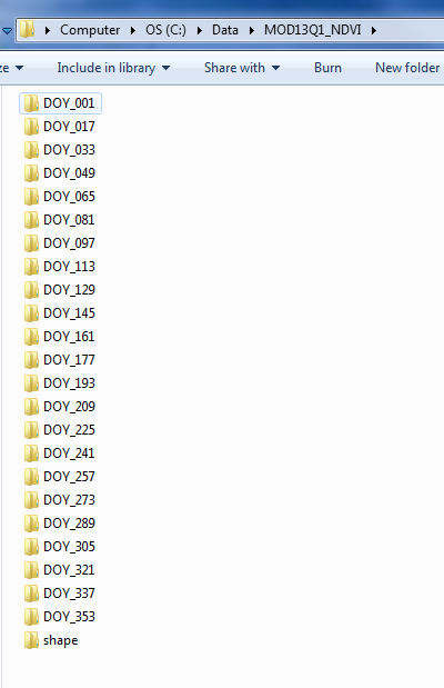
- Create one folder, where you will store all data, e.g. C:/Data.
- For each day of the year (DOY) create one subfolder. The name of each folder must start with "DOY_", e.g. DOY_033. Of course, you do not have to use data of all the avaialble days of the year. You can choose those which are most relevant in your region of interest.
- Rename the files by addding a prefix following the pattern DOY_YYYY_, e.g. 033_2001 or 001_2005, where
DOY= day of year
YYYY=year
Total Commander is a useful tool to rename multiple files: http://www.ghisler.com/index.htm).
Renaming the files is important because this pattern is used to automatize the filenames and the titles of the resulting maps in the R script.
4. Create another subfolder within the main data folder called "shape". Store the shapefile with the country border here.
Stepn 5: Download R Studio
If this is the first time for you to use R software, you will need to download and install the R software AND R Studio (whioch is an extremely useful user interface) at http://www.rstudio.com/products/rstudio/download/
Step 6: Download R Code
Download the R Code here (right click and choose "save as"). The R code is tailored to MODQ1 tif data.
Step 7: Run the R Code
1. Open R studio. 
2. Open the R script in R Studio: File - Open File.
3. Adjust the script.
Note: R uses slashes (/) for file names and not backslashes (\). R is case sensitive.
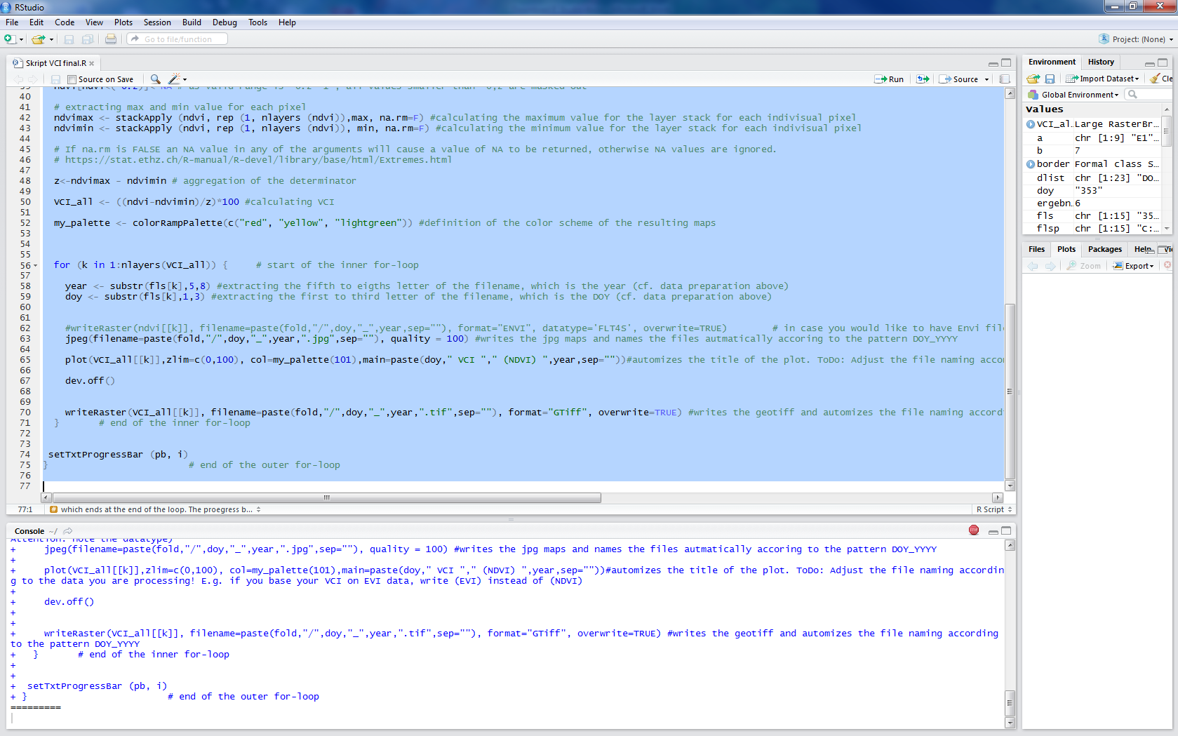
a) In line 20 border<-shapefile("C:/Data/MOD13Q1_EVI/shape/GTM_adm0.shp"), replace C:/Data/MOD13Q1_EVI/shape/GTM_adm0.shp by the link to the shapefile that you have stored on your computer.
b) Inline 23 path <- "C:/Data/MOD13Q1_EVI", replace C:/Data/MOD13Q1_EVI by the link to folder where you have stored the MODIS data.
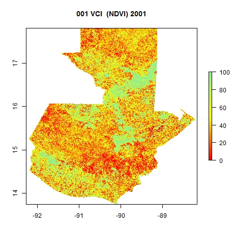
c) In line 65 plot(VCI_all[[k]],zlim=c(0,100), col=my_palette(101),main=paste(doy," VCI "," (NDVI) ",year,sep="")). adjust the file naming according to the data you are processing. E.g. if you base your VCI on EVI data, write (EVI) instead of (NDVI).
3. Install the raster package and the rgdal package by highlighting the respective text in the code (cf. figure below) and typing CTR+Enter.

4. Now, run the remaining code by highlighting it and typing CRT+Enter. depending on the size of your data, it will take quite a while (up to several hours) for the skript to run - so be patient. After a while, a progress bar will be displayed in the console. Be patient, it might take a while for the progress bar to appear. It looks like this:
======
In case you get an error message "Error: cannot allocate vector of size ... Mb" it might be that you do not have enough RAM. It is recommended to use a 64-bit operating system, and not a 32-bit system.
Another problem could be that there might not be enough space on your harddisk for the temporary files. You can either delete the temporary files manually or change the temp directory to a drive with more storage capacity by typing: rasterOptions(tmpdir="D:/temp/R_raster_temp"), where "D:/temp/R_raster_temp" of course has to be replaced by the path of your choice.
If you need to stop the skript, you can do so by clicking on the red Stop sign on the top right of the Console.
The results will be stored in the respective DOY folders as jpg (quicklook) and as tif. They are named "DOY_YYYY".
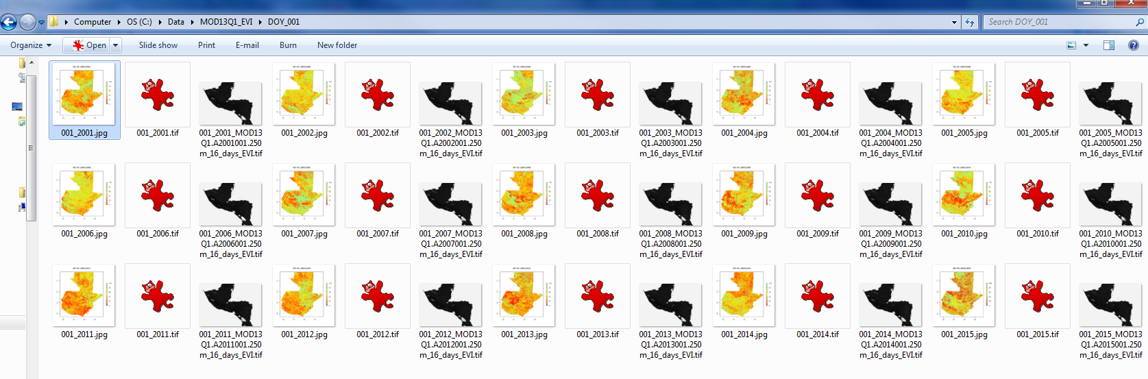
The title of the jpeg maps is following the pattern "DOY VCI (NDVI) YYYY", where DOY and YYYY are automatically adjusted according to the input data and (NDVI) can be adjusted manually in the script (cf. above). See below an example of the resulting jpeg map: