Step by step: Burn Severity with Python and optical data (Sentinel-2)

The aim of this step-by-step procedure is the generation of a burn severity map for the assessment of the areas affected by wildfires. The Normalized Burn Ratio (NBR) is used as it was designed to highlight burned areas and estimate burn severity and it uses near-infrared (NIR) and shortwave-infrared (SWIR) wavelengths. Healthy vegetation before the fire has very high near-infrared reflectance and low reflectance in the shortwave infrared part of spectrum in contrast to recently burned areas that have low reflectance in the near-infrared and high reflectance in the shortwave infrared band. More information about the NBR can be found here. The NBR is calculated for images before the fire (pre-fire NBR) and for images after the fire (post-fire NBR) and the post-fire image is subtracted from the pre-fire image to create the differenced (or delta) NBR (dNBR) image. dNBR can be used for burn severity assessment as areas with higher dNBR values indicate more severe damage whereas areas with negative dNBR values might show increased vegetation productivity and it can be classified according to burn severity ranges proposed by the United States Geological Survey (USGS).

Data required for this practice:

  • Sentinel 2 pre-fire NIR and SWIR images
  • Sentinel 2 post-fire NIR and SWIR images
  • Shapefile of Empedrado area, Chile
  • Anaconda 3

Download the data

Download the shapefile

The study area that was used for the recommmended practice is Empedrado Commune, located in the Province of Talca, Maule region, Chile. The shapefile was obtained through the Universidad de La Frontera, Temuco, Chile (Albers, C., 2012. Coberturas SIG para la enseñanza de la Geografía en Chile).

To download the shapefile, please click here.

Download the images

To download the images you can follow the procedure described here. In this practice Sentinel-2 data Level 1C are used. However, it is recommended to used Sentinel-2 Level 2A data, in the case that Level 2A data are available for the desired study area and period. More information about the processing levels of Sentinel-2 data can be found here

Download notebook

Download the notebook, the python code file and the environment file that are required here.

Download and install Anaconda 3

To run the following Jupyter Notebook you need python installed on your computer. We recommend downloading and installing Anaconda 3 (https://www.anaconda.com/download/) with the python 3.6 version as it includes a lot of useful packages.

Preparing the working environment

There are two possible approaches:

  • Install the required packages directly
  • Use the provided environment file to setup a new environment

1. Installing the required packages directly

The required package versions are:

  • python 3.6 or 3.7
  • gdal >= 2.3.1
  • numpy >= 1.15.0

The gdal package needs to be installed and it must have Bigtiff support; and numpy may need to be updated. For these reasons it is recommended to use the conda-forge package repository as follows:

  • Open the Anaconda Prompt by searching for it in the windows start menu.

  • Type: conda install -c conda-forge --no-pin gdal numpy and hit Enter

  • Type y and hit Enter if you are asked if you want to proceed.

Note: --no-pin is added to the install command in order to not restrict maximum package versions, and thus to avoid having certain packages be downgraded when installing gdal. If gdal and/or numpy do not meet the version requirements, then modify the install command to:

conda install -c conda-forge --no-pin gdal=2.3.1 numpy=1.15.0

2. Setup a new environment

All the relevant documentation can be found here.

Carry out the following steps in order to setup the environment:

  1. Open the Anaconda Prompt by searching for it in the windows start menu.
  2. Navigate to where you have saved the environment file: cd C:\my\path
  3. Type: conda env create -f environment.yml and hit Enter
    After Step 1 verify that the file you has downloaded has the following structure:

name: burn-severity

channels:
conda-forge
defaults
dependencies:
python=3.6
gdal=2.2.4
numpy=1.15.*
matplotlib
geopandas= 0.4.0
rasterio= 1.0.7
ipython
jupyter

The burn-severity environment should now be created. Make sure it is activated before running Jupyter or before running the script if you save it as a file (see the general documentation for how to do this).

In the case that Level 2A data are used you can proceed to the next step.

1. Top of the Atmosphere (TOA) corrections

The first step is to apply a top of the atmosphere correction. This is done in order to separate the actual reflectance that was emitted from the objects on the Earth's surface (which is what we need) from the atmospheric disturbances that are part of the reflected energy recorded by the sensor. You can find more information about the correction here.

1.1 Installing Sen2Cor

Sen2Cor is a processor for the generation of Sentinel-2 Level 2A product and it performs the atmospheric-, terrain and cirrus correction of Top-Of- Atmosphere Level 1C input data.

Download the Sen2Cor installation packages here and unzip the folder.

1.2 Atmospheric corrections

Follow the next steps to perform the atmospheric corrections.

  1. Open the Command Prompt by searching for it in the windows start menu.
  2. Navigate to the folder you unzipped: cd C:\my\path
  3. Find the path of L1C Sentinel-2 product you downloaded and type: L2A_Process.bat C:\my\L1C\path.SAFE

After this step a new folder containing the L2A data will be created in the same path as the L1C product and this product will be used for the processing.

2. Burn Severity

In this step the corrected images are used. In order to generate the burn severity map, the bands B8A and B12 are used. Thus, in the following code (after the function definitions) the bands of both pre- and post-fire images are loaded and the NBR is calculated. As it is already mentioned NBR is calculated using the NIR and SWIR bands of Sentinel-2 in this practice, using the formula shown below:

NBR = (NIR - SWIR) / (NIR + SWIR)

NBR = (B8A - B12) / (B8A + B12)

After calculating NBR for both pre and post-fire images, it is possible to determine their difference and obtain dNBR. Therefore, the difference between the NBR before and after the fire, referred to as dNBR during this practice is calculated. For that, the NBR of the post-images is subtracted from the NBR of the pre-images, as shown in the formula below:

dNBR = pre-fire NBR – post-fire NBR

In addition, the shapefile of the correspondent area (i.e. Empedrado) is used to clip the raster dNBR to obtain an image reflecting only the study area. As during this recommended practice, we are using the area of Empedrado region in Chile, the administrative boundary of the aforementioned area is used. In order to be able to clip the data, the shapefile and dNBR should be in the same projection and thus the shapefile is firt reprojected.

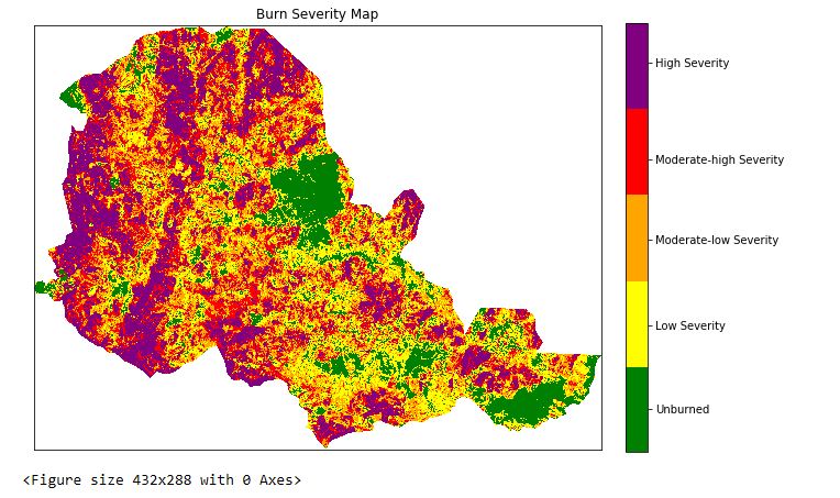
Then, USGS standard is used to classify the burn severity map according to the proposed number ranges, as explained here.

Finally, in order to quantify the area in each burn severity class, the statistics of the raster must be calculated. A transformation of the raster, so that all pixels are assigned one value for each burn severity class is necessary before the calculation.

Run this notebook using Jupyter Notebook

After downloading this notebook, start Jupyter Notebook by searching for it in the Windows start menu or by typing jupyter notebook in the Anaconda Prompt and hitting Enter. After Jupyter Notebook opened in your web browser, search for the script on your computer and open it.

Every cell has to be executed individually. A cell, which is still processing is marked by an * and a finished cell with a number. Cells are executed by clicking on the cell and hitting Shift + Enter. Alternatively, run the entire notebook sequentially (i.e. one cell at a time) click on Cell > Run All (make sure all the configuration options are set correctly).

Optional: You can run the python script (.py) either in Spyder (an IDE that comes bundled with Anaconda) or in a terminal. This may yield better performance.

The results after executing the code should look like the following figures:


Note: A cloud mask is not used in this practice, and hence if clouds are present in any of the two images it should be taken into account when assessing the burnt areas.

Note: The area calculation might include information for areas that do not represent vegetation and are misclassified, such as water bodies (e.g. river), settlements, clouds, cloud shadows, roads. Thus, in order to get more reliable results, those areas have to be masked out.

Note: In case you want to check the regrowth of the vegetation after the fire you can use two images after the fire and follow the same procedure as above and include in the classification the classes for enhanced regrowth high and low.