New User Story: Urban Tree Canopy and Impervious Surface Mapping using Google Satellite Embeddings in Los Angeles County 

Background and Issues  

Urban areas are undergoing rapid transformation as populations grow, infrastructure expands, and natural ecosystems are increasingly replaced with built environments. One of the most visible consequences of this transformation is the increase in impervious surfaces such as concrete and asphalt, accompanied by the reduction of tree canopy and vegetated spaces. This imbalance has multiple cascading effects: it intensifies the urban heat island (UHI) effect, worsens air quality, accelerates stormwater runoff, and erodes the ecosystem services that urban residents rely on for health and well-being.  

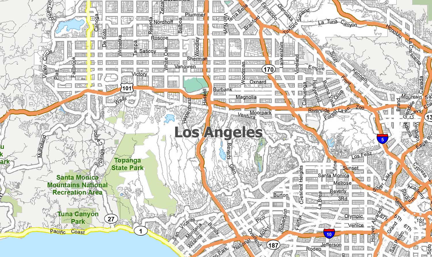
In Los Angeles County, these issues are particularly acute. With a population of more than 10 million and a wide range of land use types, the county combines dense urban cores, suburban sprawl, industrial areas, and natural mountain ranges. The region faces recurring heatwaves, smog events, and persistent inequities in access to green spaces. Addressing these challenges requires spatially explicit, up-to-date, and fine-grained information about the distribution of vegetation and impervious areas.  

Existing resources such as the National Land Cover Database (NLCD) provide valuable baseline information but are limited in two respects: they are updated only every five years, and they have a resolution of 30 meters, which is insufficient to capture small-scale urban changes such as new developments or loss of street-level greenery. These limitations are especially problematic in fast-growing metropolitan regions where timely and fine-scale monitoring is essential. Recent studies have shown that NLCD’s moderate resolution often underestimates tree canopy cover and struggles to represent heterogeneous urban landscapes (Corro et al., 2025). This creates an urgent need for more accurate, frequent, and scalable mapping approaches to better support urban planning and climate adaptation efforts.  

Technology: Satellite Embeddings  

To overcome the limitations of traditional imagery-based workflows, this project relies on the Google Satellite Embedding Dataset (V1 Annual), a cutting-edge data product developed through self-supervised learning techniques. Unlike raw satellite imagery that contains only spectral reflectance values, embeddings provide a high-level representation of the Earth’s surface.  

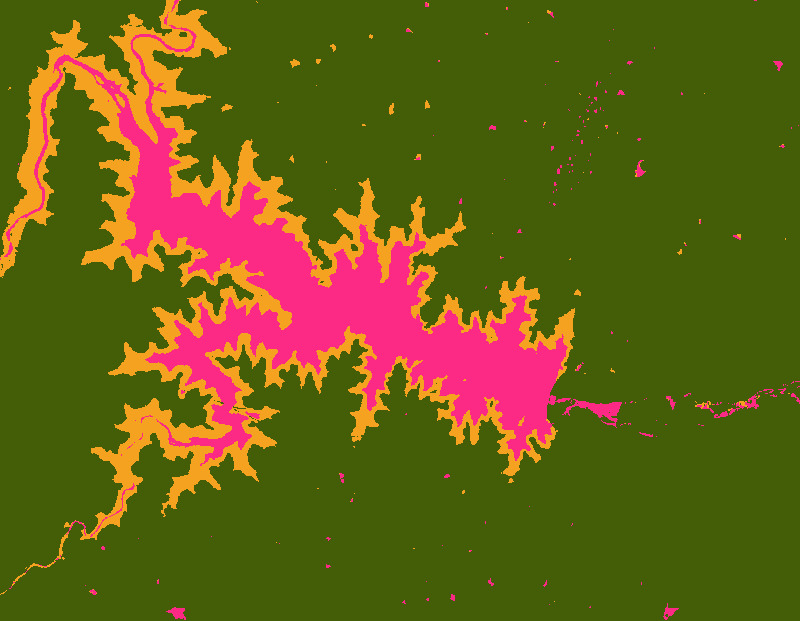
Satellite embeddings can also be better understood through visual examples provided in the Google Earth Engine tutorials. One approach is to display three of the 64 embedding bands as an RGB composite, offering a simplified view of the high-dimensional embedding space.  

What are Satellite Embeddings?  

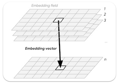
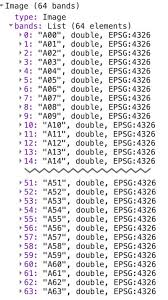
Satellite embeddings are vectors of numerical values that summarize the appearance and temporal behavior of a pixel over the course of a year. Each pixel in the embedding dataset is represented by a 64-dimensional vector, which has been derived from multi-sensor satellite data, including inputs from Landsat, Sentinel, and radar observations. By compressing this wealth of raw spectral and temporal information into a compact numerical description, embeddings capture complex patterns such as vegetation phenology, texture, and land-use characteristics that are difficult to discern from raw imagery alone. 

One of the major benefits of satellite embeddings is that they significantly reduce storage requirements and computation time, as they eliminate the need to repeatedly process large volumes of raw satellite data. Instead, researchers can work directly with compact vectors, allowing for faster analysis and efficient large-scale modeling. Moreover, because these embeddings are pre-computed from harmonized global datasets, they provide a consistent and standardized input for global studies. However, it’s important to note that the quality and representativeness of embeddings are often higher in the Global North, where data density, sensor coverage, and cloud-free observations are more abundant during the embedding construction process. This makes them particularly powerful for large-scale research and applications in regions with rich satellite data availability. 

Satellite embeddings can also be better understood through visual examples provided in the Google Earth Engine tutorials. One approach is to display three of the 64 embedding bands as an RGB composite, offering a simplified view of the high-dimensional embedding space.  

In addition, it also shows how embeddings are contextualized with cloud-masked Sentinel-2 annual composites (e.g., 2024), which highlight the multisensory inputs used to construct the embedding dataset.  

Beyond visualization, unsupervised clustering can be applied directly to the embeddings, grouping pixels with similar temporal and spectral signatures into coherent clusters. With only a few clusters, this reveals broad differences such as vegetation, water, and impervious surfaces, while increasing the number of clusters refine the segmentation into more specific land-cover types.  

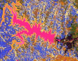
These examples highlight the capacity of satellite embeddings to represent both spatial context and seasonal variability, making them a powerful tool for urban land-cover mapping.  

Why are they useful for urban mapping?  
The value of embedding lies in its ability to reduce reliance on extensive labeled datasets. In many urban mapping projects, acquiring large volumes of ground-truth data is costly, time-consuming, and often impractical. With embeddings, classifiers can be trained using a relatively small set of labeled samples, because the embeddings themselves already contain rich spatial and temporal features. This reduces the burden on analysts while improving classification accuracy.  

Moreover, because embeddings are pre-computed and available every year, they can be accessed quickly within Google Earth Engine, allowing practitioners to focus on analysis rather than preprocessing. This opens the door to scalable, repeatable workflows that can be applied across multiple regions or years with minimal adaptation.  

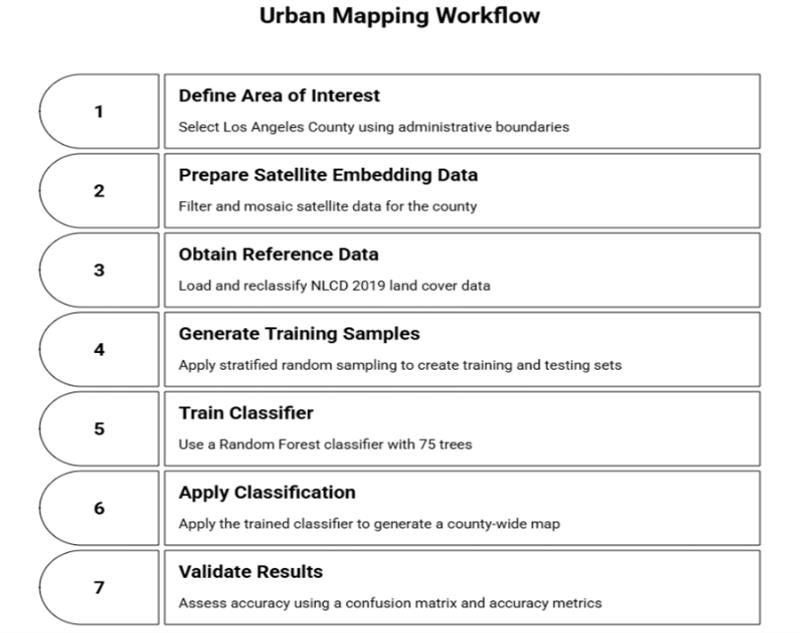
Operational Workflow  

The operational workflow developed for this project demonstrates how embeddings can be applied to real-world urban mapping challenges. The study begins by defining the area of interest, which is Los Angeles County, using publicly available administrative boundaries. The Satellite Embedding dataset is then filtered by date, restricted to the county boundary, and mosaicked to generate a single seamless image representing the year 2021.  

To train a classifier, reference data is drawn from the 2019 NLCD land cover product, which is reclassified into four categories relevant to urban studies: tree canopy, grassland/herbaceous cover, bare soil, and impervious surfaces. Stratified random sampling ensures balanced representation of each class, with 200 samples selected per category. The dataset is then split into training and testing subsets to enable validation.  

A Random Forest classifier with 75 trees is trained on the 64 embedding bands using the training samples. The classifier is subsequently applied to the embedding image, producing a county-wide classification map. Validation is performed using the test set, with results expressed as a confusion matrix, overall accuracy, and per-class accuracy measures. 

Example Implementation: Los Angeles County  

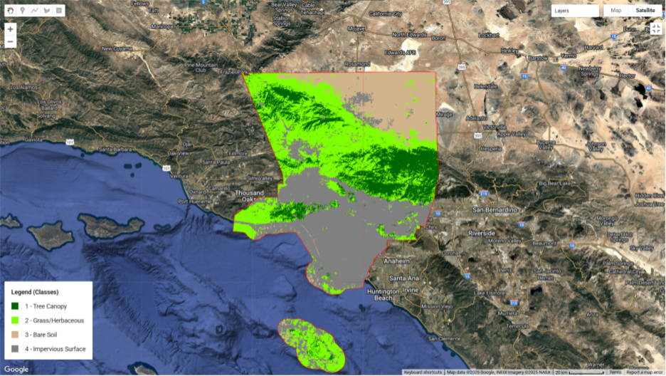
The implementation for Los Angeles County successfully produced a high-resolution map distinguishing the four target classes. The results reveal clear spatial patterns that align with known urban and ecological structures:  

• Tree Canopy is most prominent in the mountainous regions, parklands, and wealthier suburban neighborhoods where urban forestry initiatives have historically been stronger. 
• Grassland/Herbaceous Cover appears in recreational parks, open spaces, and transitional areas at the urban-rural interface. 
• Bare Soil is primarily observed in undeveloped zones on the fringes of the county and in dryland environments. 
• Impervious Surfaces dominate the dense urban core, major transport corridors, and industrial sectors. 

The classification achieved strong overall accuracy, confirming that embeddings provide sufficient information to differentiate between these classes even with a modest number of training samples. The confusion matrix highlights particularly high accuracy for impervious and tree canopy classes, while some misclassification occurred between grass and bare categories, which is a common challenge in semi-arid environments.  

Table 1. Confusion matrix of classification results  

Google Earth Engine Code 

https://code.earthengine.google.com/50a196d87d4a22f2fd2e5fa20db9182e 

Google Earth Engine Code for embedding-based classification in Los Angeles County. 

// ----------------------------- 
// Urban Tree / Grass / Bare / Impervious Mapping 
// Los Angeles County, 2021 
// ----------------------------- 
 
// 1. Study Area: Los Angeles County (TIGER dataset) 
var laCounty = ee.FeatureCollection("TIGER/2018/Counties") 
  .filter(ee.Filter.eq("NAME", "Los Angeles")) 
  .geometry(); 
 
Map.centerObject(laCounty, 9); 
Map.addLayer(laCounty, {color: 'red'}, "LA County Boundary"); 
 
// 2. Satellite Embeddings (Annual 2021) 
var year = 2021; 
var embeddingsIC = ee.ImageCollection("GOOGLE/SATELLITE_EMBEDDING/V1/ANNUAL") 
  .filterDate(year + "-01-01", (year + 1) + "-01-01") 
  .filterBounds(laCounty); 
 
print("Embedding tiles found:", embeddingsIC.size()); 
 
var embeddings = embeddingsIC.mosaic().clip(laCounty); 
print("Embedding bands (64):", embeddings.bandNames()); 
 
// 3. Reference Data: NLCD 2019 
var nlcd = ee.Image("USGS/NLCD_RELEASES/2019_REL/NLCD/2019") 
  .select('landcover') 
  .clip(laCounty); 
 
// 4. Define Classes (Tree=1, Grass=2, Bare=3, Impervious=4) 
var tree = nlcd.eq(41).or(nlcd.eq(42)).or(nlcd.eq(43)); 
var grass = nlcd.eq(71); 
var bare = nlcd.eq(31); 
var impervious = nlcd.eq(22).or(nlcd.eq(23)).or(nlcd.eq(24)); 
 
var validMask = tree.or(grass).or(bare).or(impervious); 
 
var trainingMask = tree.multiply(1) 
  .add(grass.multiply(2)) 
  .add(bare.multiply(3)) 
  .add(impervious.multiply(4)) 
  .updateMask(validMask) 
  .rename('class') 
  .toByte(); 
 
// 5. Stratified Sampling (200 per class) 
var trainingPoints = trainingMask.stratifiedSample({ 
  numPoints: 0, 
  classBand: 'class', 
  classValues: [1, 2, 3, 4], 
  classPoints: [200, 200, 200, 200], 
  region: laCounty, 
  scale: 30, 
  seed: 42, 
  geometries: true 
}); 
 
print("Sample sizes by class:", trainingPoints.aggregate_histogram('class')); 
 
// 6. Train/Test Split 
var withRandom = trainingPoints.randomColumn('random', 42); 
var trainSet = withRandom.filter(ee.Filter.lt('random', 0.7)); 
var testSet  = withRandom.filter(ee.Filter.gte('random', 0.7)); 
 
// 7. Train Classifier (Random Forest, 75 trees) 
var bands = embeddings.bandNames(); 
var training = embeddings.sampleRegions({ 
  collection: trainSet, 
  properties: ['class'], 
  scale: 10, 
  tileScale: 4 
}); 
 
var classifier = ee.Classifier.smileRandomForest(75).train({ 
  features: training, 
  classProperty: 'class', 
  inputProperties: bands 
}); 
 
// 8. Classify Entire County 
var classified = embeddings.classify(classifier).clip(laCounty); 
 
// 9. Accuracy Assessment 
var testing = embeddings.sampleRegions({ 
  collection: testSet, 
  properties: ['class'], 
  scale: 10, 
  tileScale: 4 
}); 
 
var validated = testing.classify(classifier); 
var confMatrix = validated.errorMatrix('class', 'classification'); 
 
print('Confusion Matrix:', confMatrix); 
print('Overall Accuracy:', confMatrix.accuracy()); 
 
// 10. Visualization (County-wide) 
var palette = ['006400', '7FFF00', 'D2B48C', '808080'];  
Map.addLayer(classified, {min: 1, max: 4, palette: palette}, 
             'Tree/Grass/Bare/Impervious'); 
 
// 11. Add Legend 
function addLegend() { 
  var legend = ui.Panel({style: {position: 'bottom-left'}}); 
  legend.add(ui.Label({value: 'Legend (Classes)', style: {fontWeight: 'bold'}})); 
  var names = ['Tree Canopy', 'Grass/Herbaceous', 'Bare Soil', 'Impervious Surface']; 
  for (var i = 0; i < 4; i++) { 
    legend.add(ui.Panel([ 
      ui.Label({style: {backgroundColor: '#' + palette[i], padding: '8px'}}), 
      ui.Label({value: (i+1) + " - " + names[i]}) 
    ], ui.Panel.Layout.Flow('horizontal'))); 
  } 
  Map.add(legend); 
} 
addLegend(); 

Conclusion  

This case study demonstrates the practical potential of satellite embeddings to transform urban land cover mapping. By compressing raw multi-sensor imagery into rich numerical vectors, embeddings allow practitioners to bypass many of the limitations of traditional workflows. They make it possible to classify large urban regions with fewer training samples, at higher resolution, and with improved efficiency. 

For Los Angeles County, the resulting maps provide a clear and accurate picture of where vegetation and impervious surfaces are distributed. This information directly supports urban heat island mitigation strategies, green infrastructure planning, and equitable access to urban greenery. Beyond LA, the workflow is easily transferable to other regions, making it a valuable practice for global applications. 

In cities across developing countries, this approach offers a powerful, low-cost alternative to conventional land cover mapping methods that often require extensive ground surveys and high-end computing resources. Since the embedding-based workflow can be implemented using freely available satellite data and cloud platforms like Google Earth Engine, local governments and researchers can generate detailed urban land cover maps with limited infrastructure. This enables evidence-based decision-making for urban planning, climate resilience, and sustainable development in rapidly growing metropolitan areas where data scarcity has traditionally hindered progress. 

Future Directions  

The embedding-based workflow presented here has significant potential for scaling and adaptation. Future applications could focus on producing multi-year time series to monitor how tree canopy and imperviousness change over time, enabling the detection of trends and rapid response to urbanization pressures. Another avenue is to integrate embedding-based maps with socio-economic and health data to support policy decisions that prioritize the most vulnerable communities.  

Reference 

Corro, S. V., Behnamian, A., McGovern, A., Mueller, M., Stewart, J. S., Arndt, S. A., & Wimberly, M. C. (2025). Harmonized 30 m impervious surface time series for the conterminous United States, 1985–2020. Scientific Data, 12(1), 174. https://gee-community-catalog.org/projects/us_tcc/   

GIS Geography. (n.d.). Los Angeles map, California. Retrieved September 12, 2025, from https://gisgeography.com/los-angeles-map-california/  

Google Earth Engine / spatialthoughts. (n.d.). Introduction to the Satellite Embedding Dataset [Tutorial]. Google Developers. Retrieved September 12, 2025, from https://developers.google.com/earth-engine/tutorials/community/satellite-embedding-01-introduction  

Google Earth Engine & Google DeepMind. (n.d.). Satellite Embedding V1 Annual [Dataset]. Google Developers. Retrieved September 12, 2025, from https://developers.google.com/earth-engine/datasets/catalog/GOOGLE_SATELLITE_EMBEDDING_V1_ANNUAL