Pratique recommandée: Cartographie des inondations

Tereza D Thu, 6 Apr 2017 - 14:55

Cette pratique recommandée se consacre à l’usage de l’imagerie satellite SAR pour la cartographie des inondations. La pratique montre l’usage du logiciel SNAP d’ESA pour le pré-traitement et le traitement de l’imagerie SAR en utilisant la technique de seuillage pour dériver l’extension des inondations. Pour visualiser les résultats du traitement d’images, Google Earth est utilisé. Cette pratique a été développée par l’Institute de la recherche spatiale NASU-SSAU, Ukraine.

Pas à pas Inondations

En détail Inondations

Objective

L’objectif de cette pratique est de déterminer l’extension de l’espace inondé. L’usage de l’imagerie satellite SAR pour la cartographie d’extension des eaux présente une solution viable pour traiter les images rapidement en fournissant l’information en temps quais réel sur l’inondation aux agences de secours. En plus, l’information sur l’extension des eaux peut être utilisée pour l’évaluation des dégâts et pour la gestion des risques, créant les scénarios qui montrent la population, l’activité économique et l’environnement exposés au risque d’inondation.

Disaster type

Inondation

Disaster Cycle Phase

Relief & Response

Test Site

Malawi

Context

La pratique a été utilisée dans le cas des inondations au Malawi en janvier 2015. À partir de décembre 2014, Malawi a été affecté par des pluies battantes qui ont causé le débordement des fleuves. La pratique recommandée a été utilisée dans la zone affectée à Chiromo dans le district Nsanje.

Applicability

Cette pratique peut être utilisée globalement. Elle a été utilisée avec succès dans le cas des inondations en Australie, Afrique et Asie. La condition préalable pour la détection d’eau sur des images SAR est une rugosité de surface très faible. Une fausse alerte peut se produire dans le cas des zones où il y a l’ombre radar due au terrain variable ou aussi dans le cas où des objets lisses, comme par exemple les routes ou le sable, sont présents. La détection des inondations dans les zones urbaines reste alors difficile. La détection de la végétation inondée par imagerie SAR exige une approche différente qui utilise deux images multi-temporelles.

en_detail_0.pdf (465.54 KB)

pas_a_pas_0.pdf (3.92 MB)

In Detail: Recommended Practice Flood Mapping

/advisory-support/recommended-practices/recommended-practice-flood-mapping

anne.pustina Thu, 6 Feb 2014 - 16:16

/advisory-support/recommended-practices/recommended-practice-flood-mapping/vers…

Abstract

Efficient monitoring and prediction of floods and risk management for a large river is quasi-impossible without the use of Earth Observation (EO) data from space. As a matter of fact, one of the most important problems associated with flood monitoring is the difficulty to determine the extent of the flood area as even a dense network of observations cannot provide such information. The flood extent information is used for damage assessment and risk management, and benefits to rescuers during flooding; it is also very important for calibration and validation of hydraulic models to reconstruct what happened during the flood and determine what caused the water to go where it did.

SAR (synthetic aperture radar) measurements from space are independent of daytime and weather conditions and can provide valuable information to monitoring of flood events. This is mainly due to the fact that smooth water surface provides no return to the antenna in microwave spectrum and appears black in SAR imagery. SAR data produces a result with limited accuracy in densely populated areas due to the increased amount of backscattering from houses and other objects. In such cases, the use of optical data is advantageous and can be found here.

However, this recommended practice focuses on a simple threshold method for deriving flood extent from SAR imagery.

Requirements

Data requirements: SAR images (current and possible archived) in Level1, and DEM for ortho-rectification. (SRTM DEM is automatically downloaded in SNAP within orthorectification procedure) Also, archived optical imagery, land cover/land use maps with vector data on infrastructure objects are beneficial.
For SAR image processing, both 32 and 64-bit versions of SNAP are freely available from http://step.esa.int/main/download/ (registration required). For visualization, we will use Google Earth which can be freely downloaded from https://www.google.com/earth/explore/products/.
Skills requirements: basic to intermediate knowledge of image processing; basic knowledge of SAR theory.
Hardware requirements: for processing real SAR images, it is advisable to have minimum 2 GB of RAM. Use of multi-core processors (with hyperthreading) is beneficial since SNAP is parallelised.

Applications

The applications of flood extent include:

Operational estimation and detection of flooded areas (within 6-12 h after data acquisition).
Damage assessment of flooded objects.
Calibration of hydrometeorological models.
Detection of water levels using high-resolution DEM.
Spatial extent: from villages to a global scale.
Can be used for all stages: risk assessment, operational mapping and response, recovery.
Spatial resolution: from 1 m to 150 m.

Strengths and Limitations

The use of the threshold method for SAR has the following advantages:

Cloud independent SAR images.
High revisit time.
Easy detection of smooth water.
Accuracy: up to 95% (depending on the landscape and area).

Limitations:

Potential false alarm from shadows (variable terrain), smooth objects (like roads) and sand.
Difficulties in detection floods in urban areas.
Difficulties in detecting flooded vegetation. (For flooded vegetation detection from SAR usually, two multi-temporal images are required.)

Workflow

General description of the workflow:

(0) SAR image acquisition.

(1) Calibration in SNAP through Radiometric Correction.

(2) Speckle filtering in SNAP.

(3) Binarization in SNAP through Band Math

(4) Geometric correction in SNAP through Range Doppler Terrain Correction Function.

(5) Visualization in Google Earth.

Bibliography

Kussul N., Shelestov A., Skakun S. “Flood Monitoring on the Basis of SAR Data”, In F. Kogan, A. Powell, O. Fedorov (Eds.) “Use of Satellite and In-Situ Data to Improve Sustainability”. NATO Science for Peace and Security Series C: Environmental Security, 2011, pp. 19-29. (http://dx.doi.org/10.1007/978-90-481-9618-0_3)

Kussul N., Shelestov A., Skakun S. (2008) “Grid System for Flood Extent Extraction from Satellite Images”, Earth Science Informatics, 1(3-4), pp. 105-117. (http://dx.doi.org/10.1007/s12145-008-0014-3)

Skakun S. (2010) “A Neural Network Approach to Flood Mapping Using Satellite Imagery”, Computing and Informatics, Vol. 29, No. 6, pp. 1013-1024.

Kussul N., Shelestov A., Skakun S., Guoqing Li, Kussul O., Jibo Xie, (2013) “Service-oriented infrastructure for flood mapping using optical and SAR satellite data”, International Journal of Digital Earth, (http://dx.doi.org/10.1080/17538947.2013.781242)

Kussul N., Shelestov A., Skakun S., Li G., Kussul O. (2012) “The Wide Area Grid Testbed for Flood Monitoring Using Earth Observation Data”, IEEE Journal of Selected Topics in Applied Earth Observations and Remote Sensing, 2012, vol. 5, no. 6, pp. 1746- 1751. (http://dx.doi.org/10.1109/JSTARS.2012.2201447)

Kussul N., Shelestov A., Skakun S. (2009) “Grid and Sensor Web Technologies for Environmental Monitoring”, Earth Science Informatics, 2(1-2), pp. 37-51. (http://dx.doi.org/10.1007/s12145-009-0024-9)

Step by Step: Recommended Practice Flood Mapping

/advisory-support/recommended-practices/recommended-practice-flood-mapping

jan.stefanski Fri, 25 Sep 2015 - 10:19

/advisory-support/recommended-practices/recommended-practice-flood-mapping/in-d…

Data Access

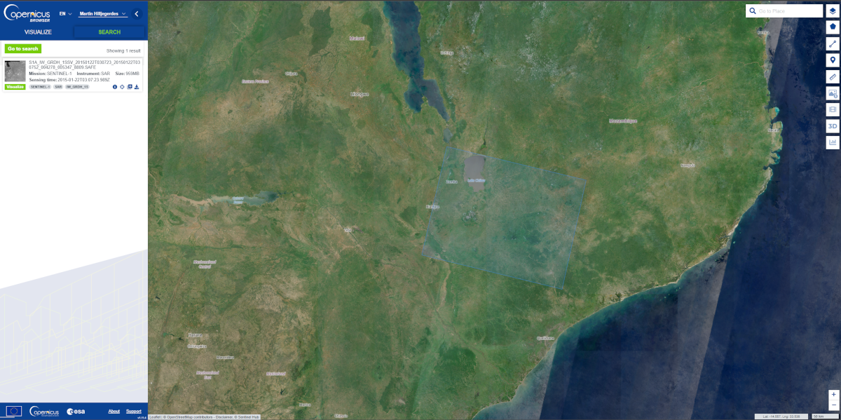
SAR data from Sentinel-1, a SAR mission from ESA, is available free of charge. To download Sentinel-1 data, register at the Copernicus Data Space Ecosystem. Then a search option becomes available which can be used to specify the data need such as region of interest, product type, sensor mode, sensing period, among others. In the example below, we used Level-1 Ground Range Detected (GRD) Sentinel-1 data, which incorporates already some basic preprocessing.

Copernicus Data Space Ecosystem

Other SAR imagery is not freely available; these include: Radarsat-2, TerraSAR-X, and Cosmo-SkyMed. But archived SAR images from past missions can be freely obtained. For example, SAR images from Envisat/ASAR can be obtained from the ESA Category-1 programme (http://eopi.esa.int/). Also, for commercial images (Radarsat-2, TerraSAR-X, and Cosmo-SkyMed) there are opportunities for scientific use of data for free or reduced rates.

Processing and screenshots are based on ESA's Sentinel Application Platform (SNAP) version 8.0 64-bit.

Step 0: Data preparation

Step 1: Pre-processing - Calibration

Step 2: Pre-processing - Speckle filtering

Step 3: Binarization

Step 4: Post-processing - Geometric correction

Step 5: Visualization in Google Earth

Example of the resulting product

Data Preparation/Pre-processing

SNAP supports all major data formats that are used to store SAR images.

0. Data preparation

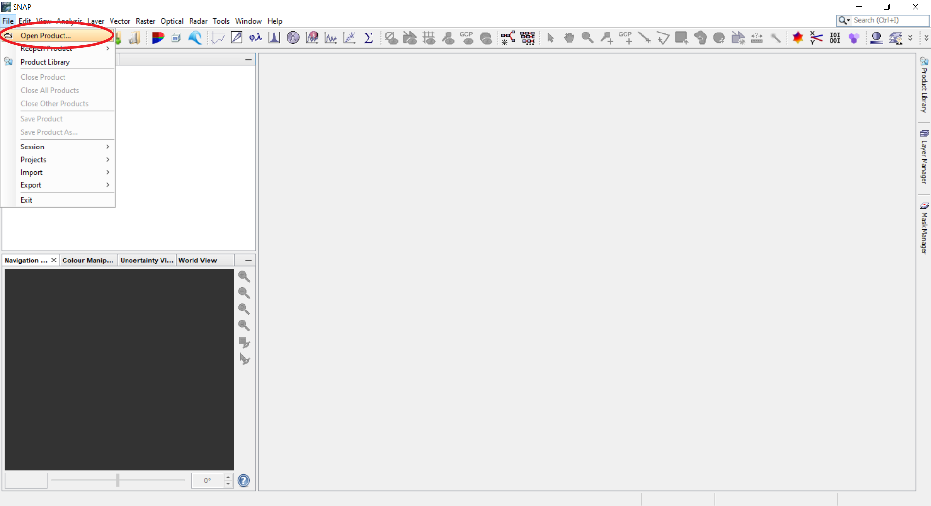
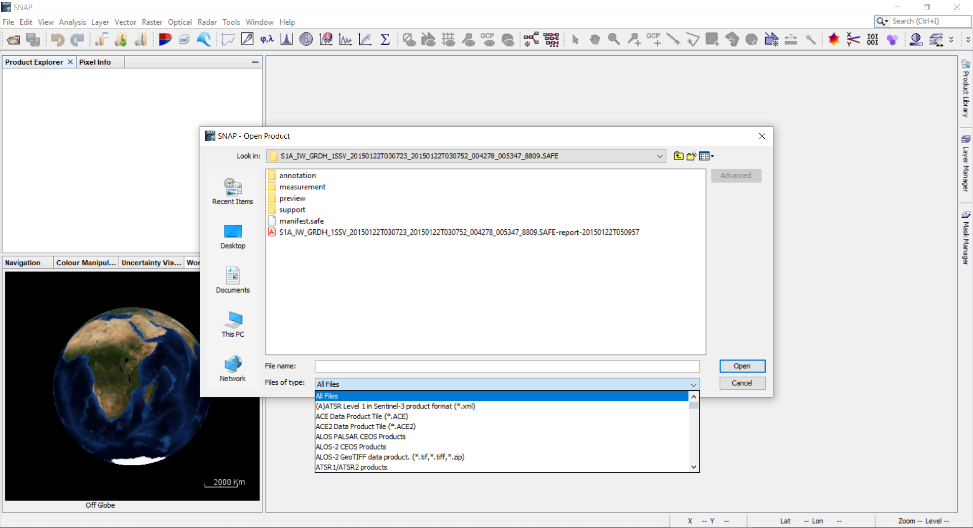
0.1 To read the data set point to File --> Open Product.

0.2 Select the Sentinel-1 image, either directly the *.zip file or the manifest.safe from the unzipped folder.

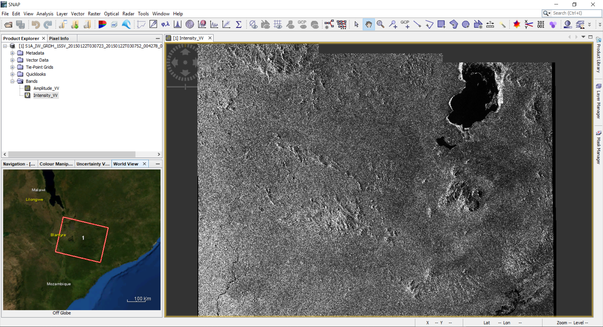
0.3 The Product Explorer on the left shows relevant information on the product. This includes: Metadata (different SAR parameters on the orbit and image); Tie-points grid (interpolated latitude, longitude, incident angle and slant range time values); Bands (actual image bands). By right clicking on the Product, Properties can be opened which include information on mission, acquisition date, pass, etc.

0.4 For each polarization recorded there are two bands: Amplitude and Intensity. (The Intensity band is a virtual one. It is the square of the amplitude). Double click on either Amplitude or Intensity to view the image. In the bottom left corner, the WorldWind View shows the footprint of the selected scene.

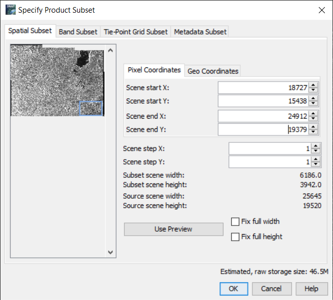
0.5 If you need a subset, select on the Menu panel Raster --> Subset. Specify parameters of the region of interest and click OK button. SNAP will open the product with all metadata relevant to the subset.

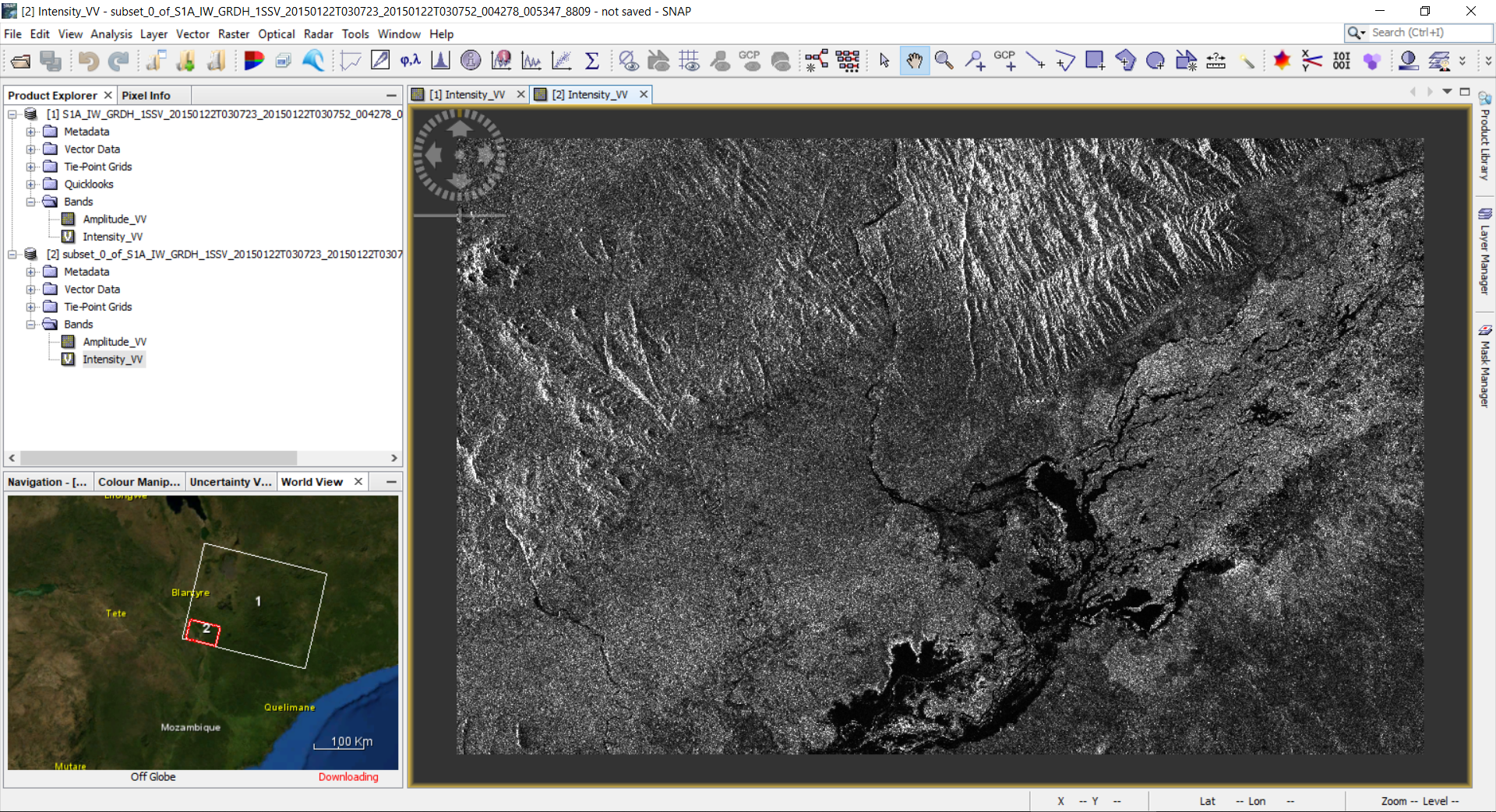
0.6 The created subset is added as a new product, which is handled simultaneously as described in step 0.4. The footprint of the subset is also shown in the WorldWind View.

1. Pre-processing - Calibration

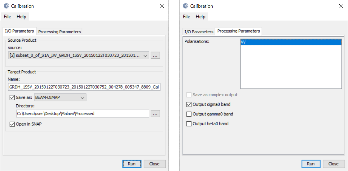
1.1 Calibration: select on the Menu panel Radar --> Radiometric --> Calibrate.

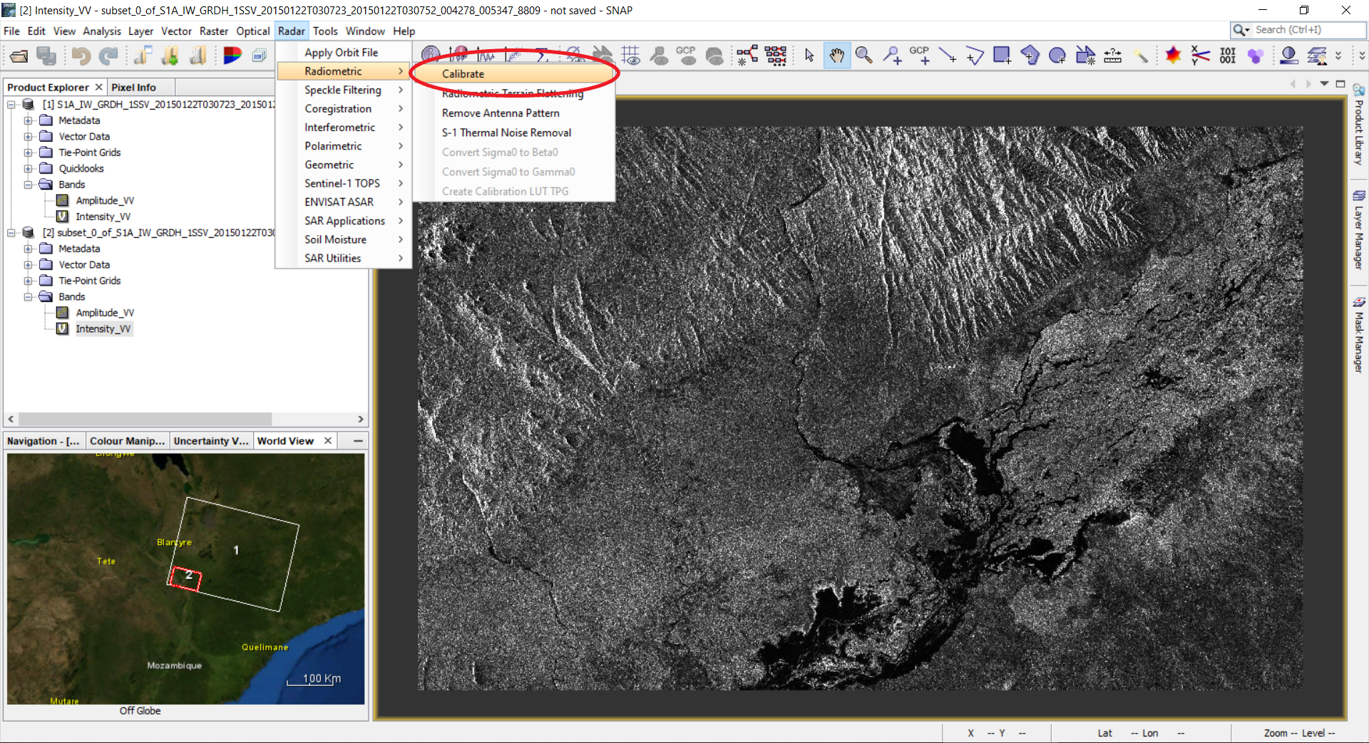
1.2 A Calibration window will open. Select the tab: Processing Parameters. Select the Polarizations you wish to process. This will create a new product with calibrated values of the backscatter coefficient.

2. Pre-processing - Speckle filtering

2.1 Next step is filtration. Select Radar --> Speckle Filtering --> Single Product Speckle Filter.

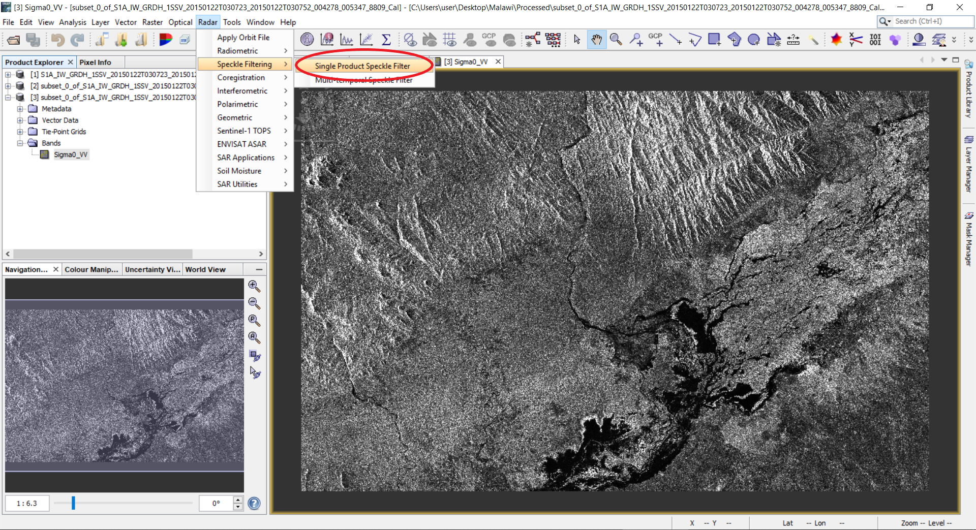
2.2 A Speckle filtering window will appear. Select the tab: Processing Parameters. Select Sigma0_VV and select Lee filter with filter size 7 by 7. Click the Run button.

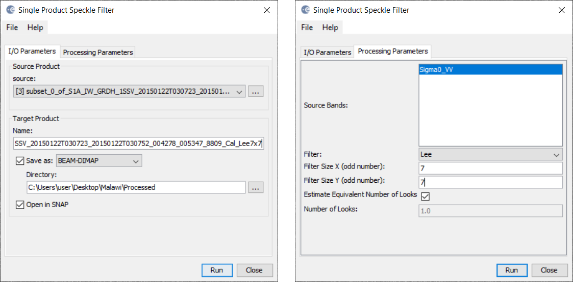
2.3 A new product will be created in the Product Explorer. Open the band in the newly created product.

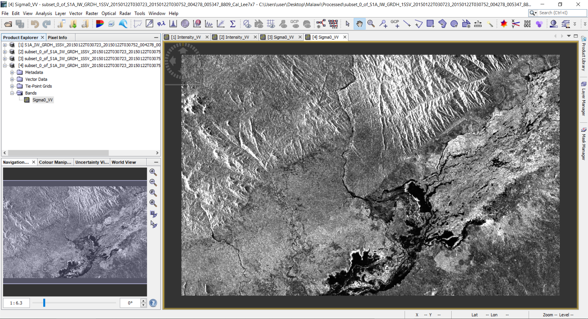
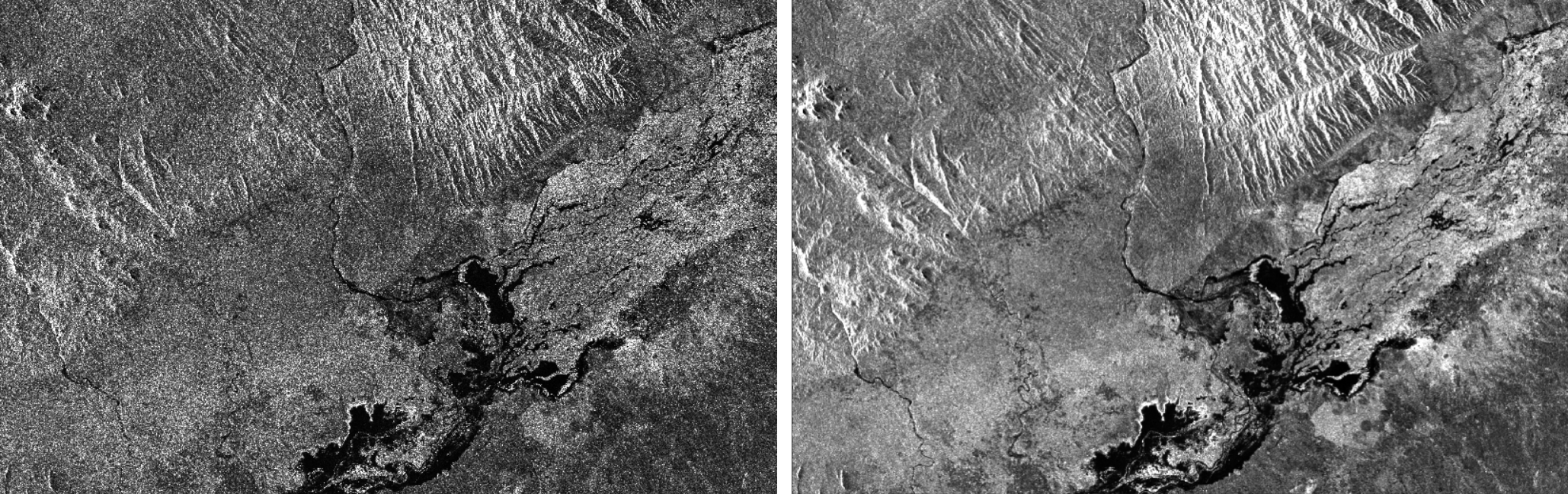
2.4 Compare the non-filtered and filtered versions.

Processing Steps

3. Binarization

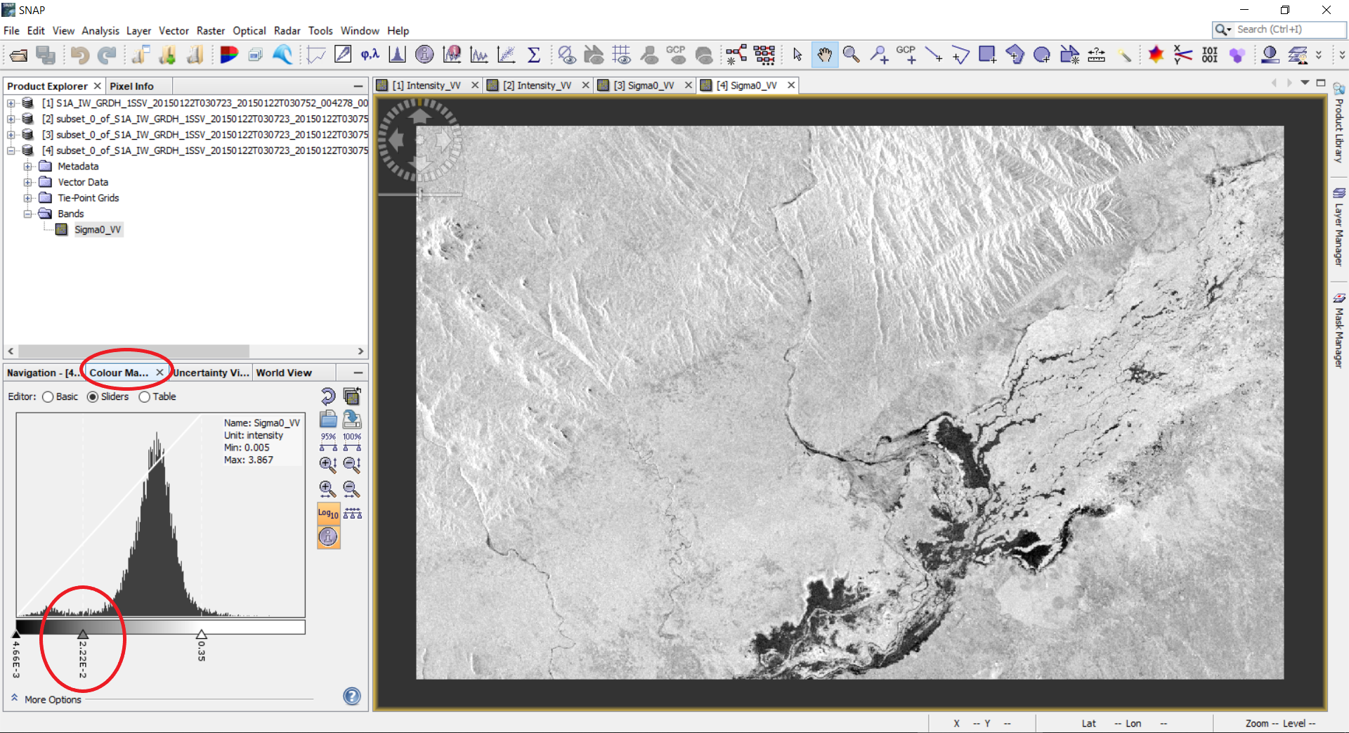
3.1 To separate water from non-water a threshold can be selected. For this, we will analyse the histogram of the filtered backscatter coefficient. On the left side panel select the Colour Manipulation tab. The histogram of the backscatter coefficient will show up and one might need to use the logarithmic display. The histogram will show one or more peaks of different magnitude depending on the data. Low values of the backscatter will correspond to the water, and high values will correspond to the non-water class. We need to select the value that will separate water from non-water. In our case, the threshold value will be 2.22E-2.

3.2 To segment or binarize the image we will apply band arithmetic. For this, go to Raster --> Band Maths…

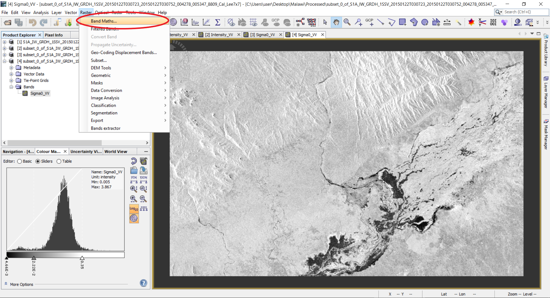
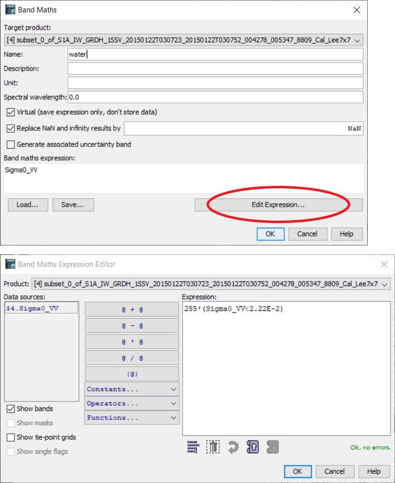
3.3 A window will open. Type a name for the new band, for example, water. Remove checkbox from the virtual band (the virtual band is in the memory but not physically on the disc). Click Edit Expression… button. The band math utility allows one to make any sorts of mathematical and logical expressions on the bands available in the product. Our goal is to create a new image which will be, for example, 255, for water objects (for backscatter lower our threshold of 2.22E-2), and 0 for higher values. To do this, enter into the Expression field the following expression: 255*(Sigma0_VV<2.22E-2). The expression (Sigma0_VV<2.22E-2) will return the logical value: true (or 1) for values less than 2.22E-2, and false (or 0) for higher values. Then we just multiply by 255. Click OK button.

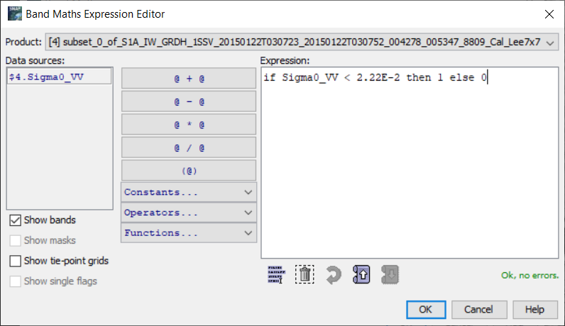
Alternatively, another Band Math equation could be

if Sigma0_VV < 2.22E-2 then 1 else 0

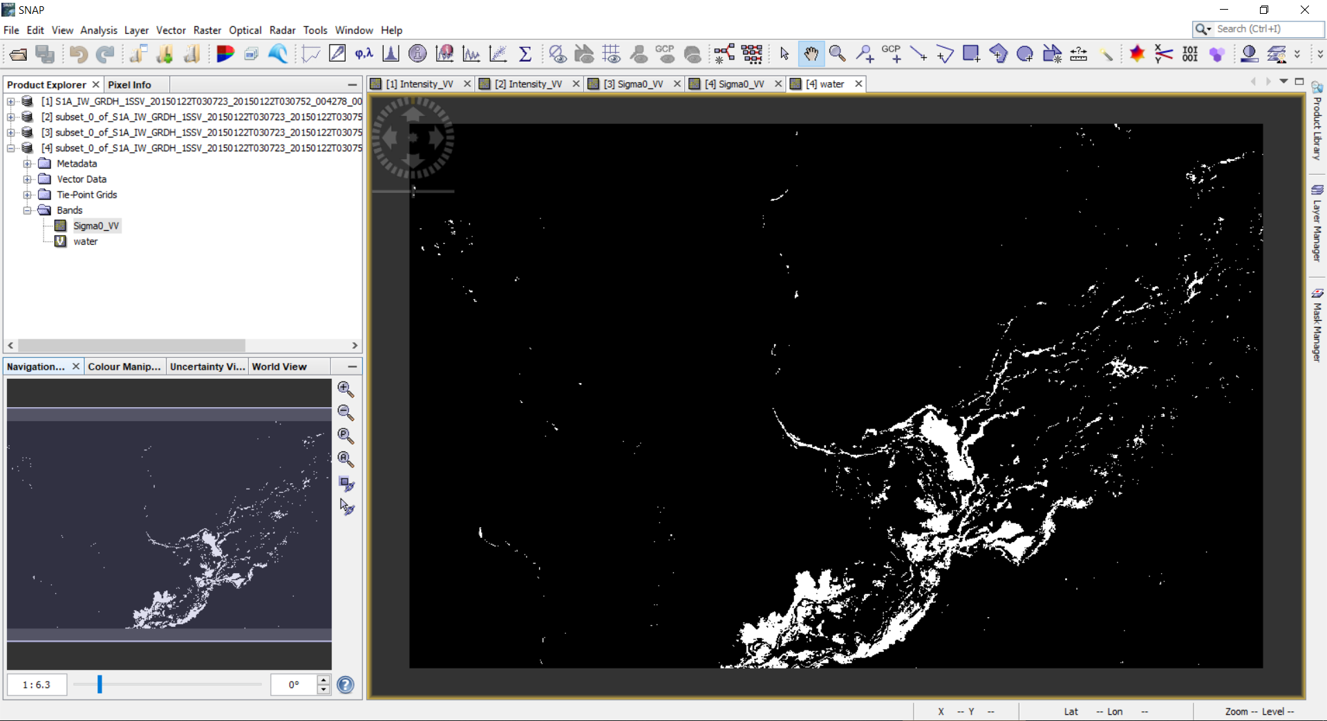
3.4 A new band named water will be added to the product. Double click this band to view the image.

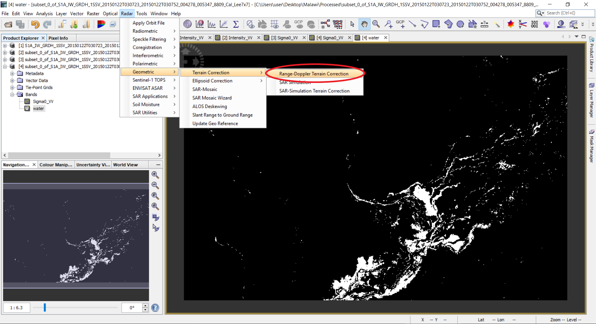
4. Post-processing - Geometric correction

4.1 The obtained image is in the geometry of the sensor. We need to reproject it to the geographic projection. To do this, select Radar --> Geometric --> Terrain Correction --> Range-Doppler Terrain Correction.

4.2 A window with parameters will open. Select the Processing Parameters tab. In the Source Bands select only water; Digital Elevation Model - SRTM 3Sec (Auto Download), the DEM over the region that SAR image covers will be automatically downloaded, use SRTM 1Sec (Auto Download) if the tool does not run properly; DEM Resampling Method - BILINEAR_INTERPOLATION; Image Resampling Method - NEAREST_NEIGHBOUR; Pixel Spacing - 10m (which depends on the sensor and its acquisition mode); Map projection - WGS84(DD), if UTM coordinates are needed, use UTM/WGS84 (Automatic), SNAP will automatically select the zones. Click OK button.

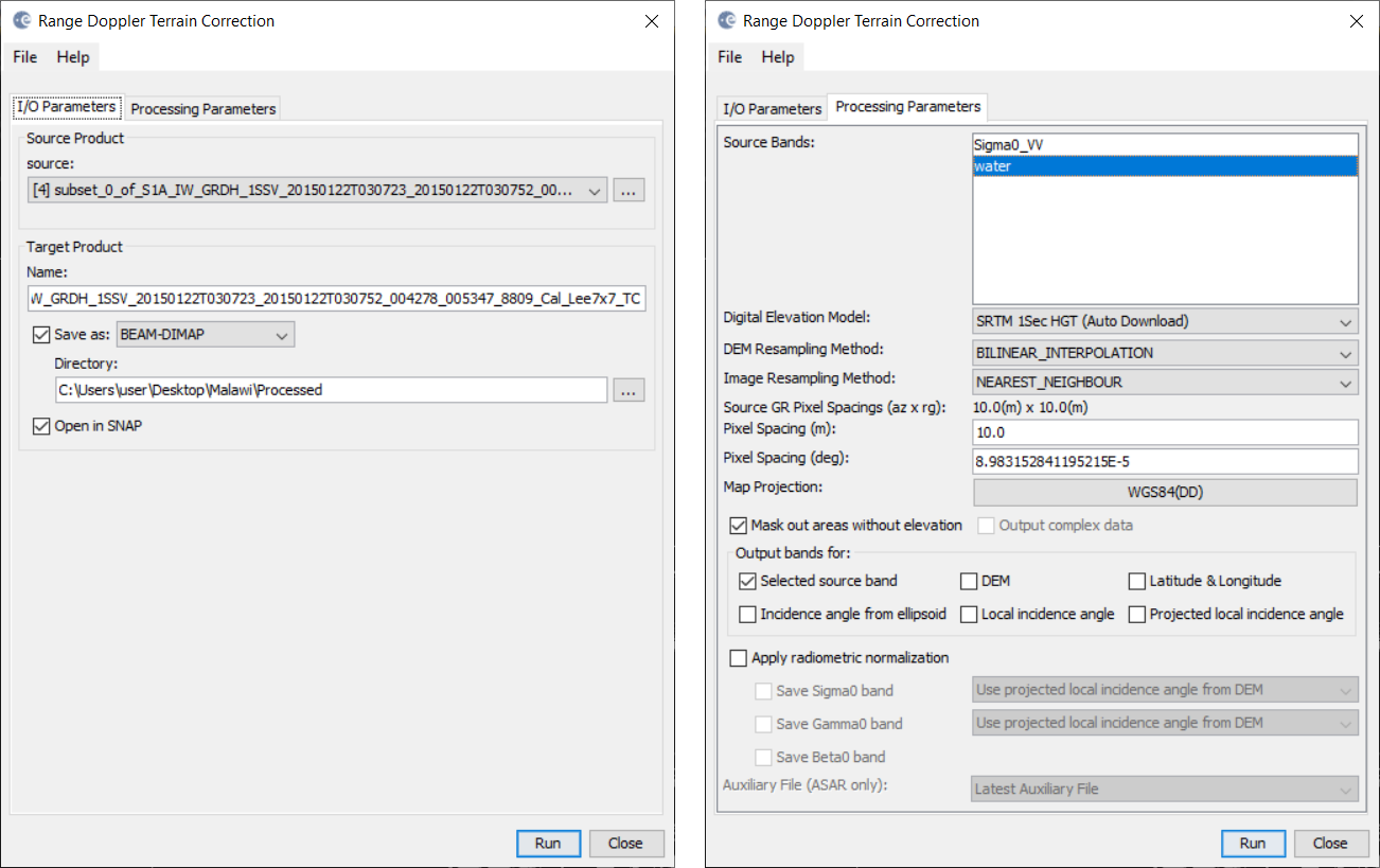
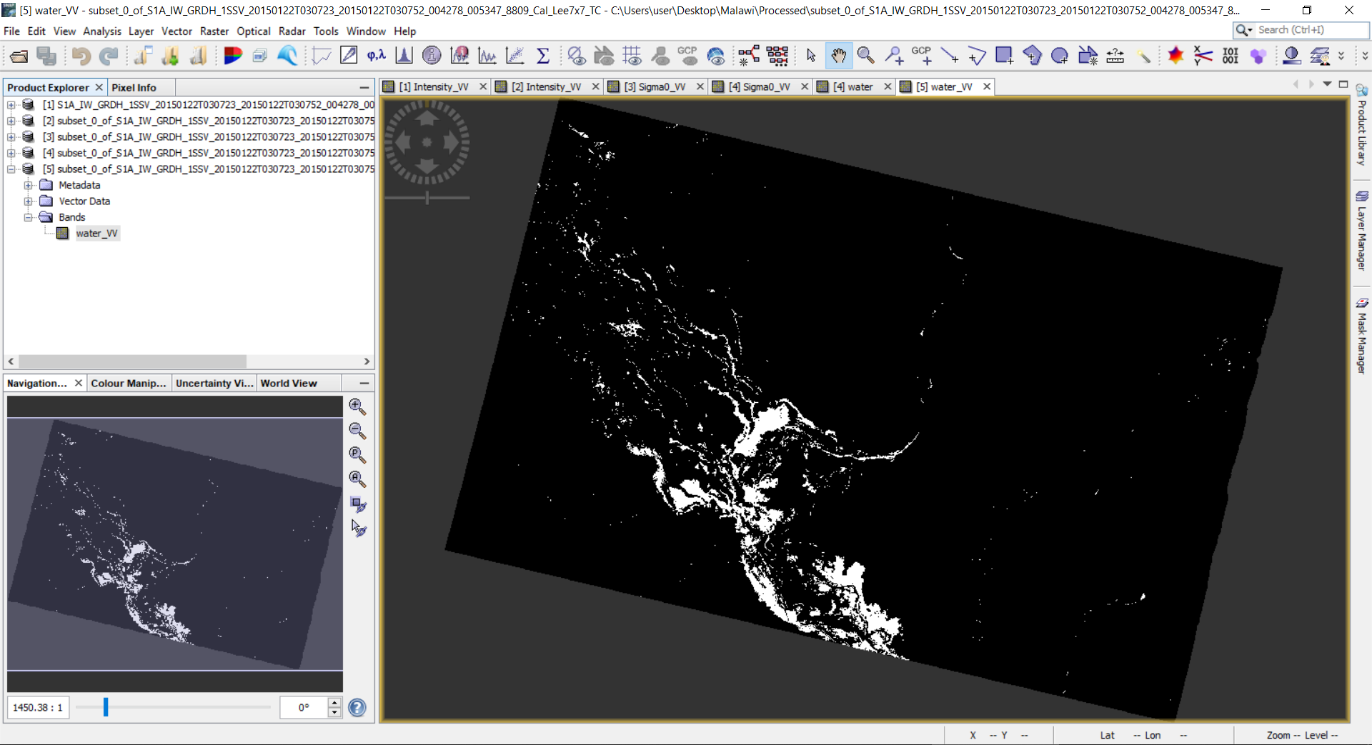
4.3 A new product will be created and appear in the Product Explorer. The product will be created in the DIM format and the image will be in img format. Double click the band in the newly created product. Notice that the geometry of the image changed to the geographic projection. This file can now be opened in a GIS (for example QGIS) to visualize and create a map.

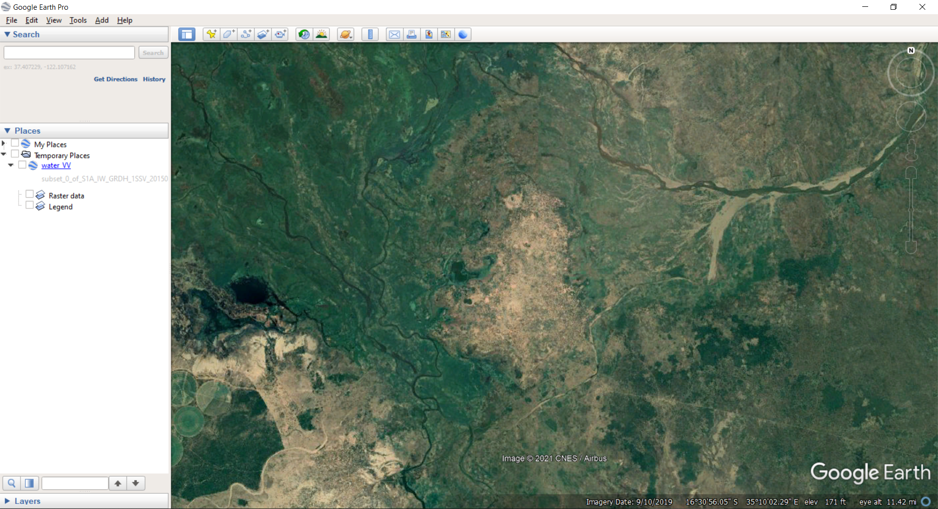
5. Visualization in Google Earth

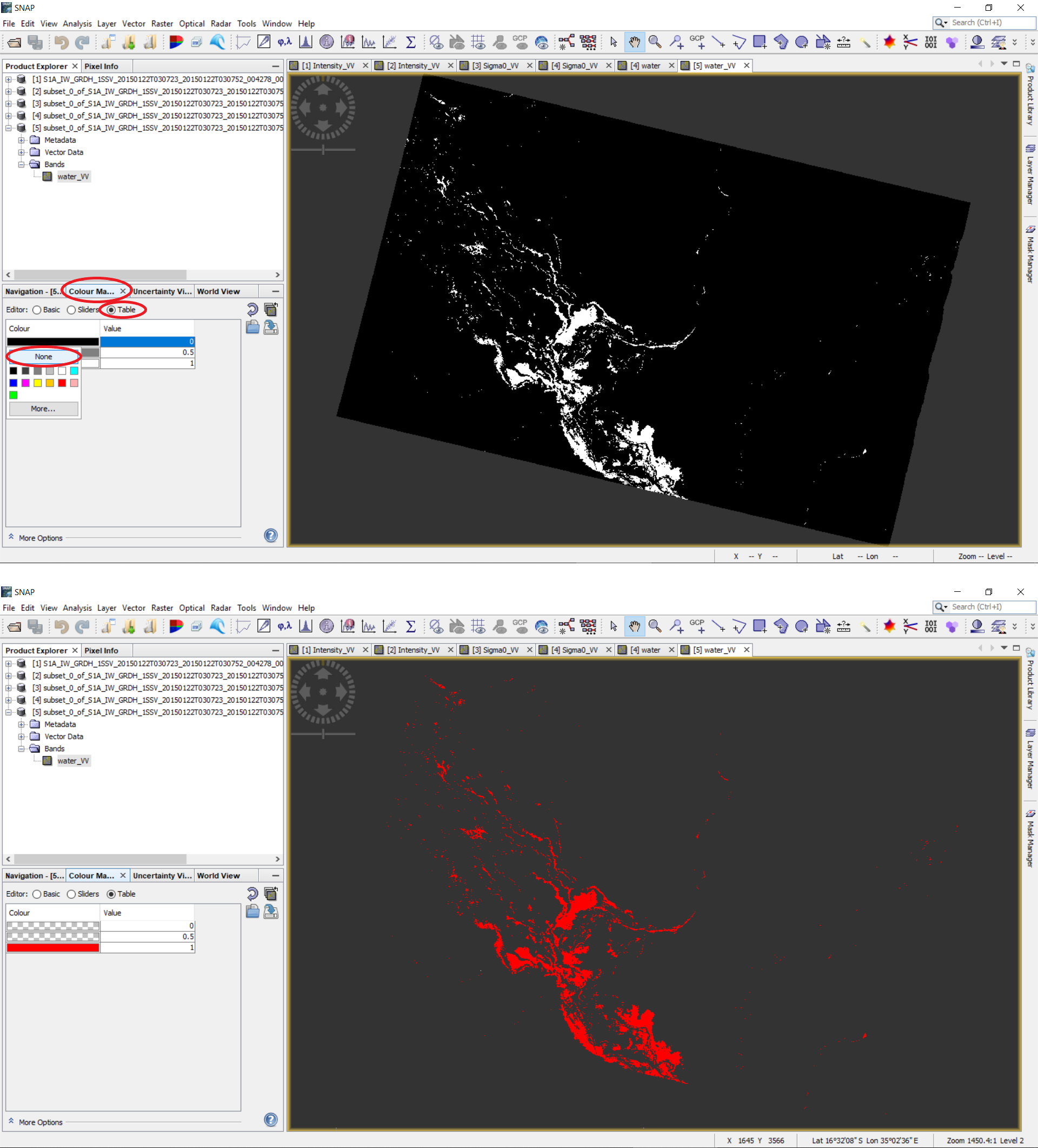
5.1 In order to display solely the water pixels, go to the left side panel, select the Colour Manipulation tab and the Table editor. Click on the boxes under Colour and set the background colours to None to make it transparent; optionally, you can change the water pixels (white colour) to another colour.

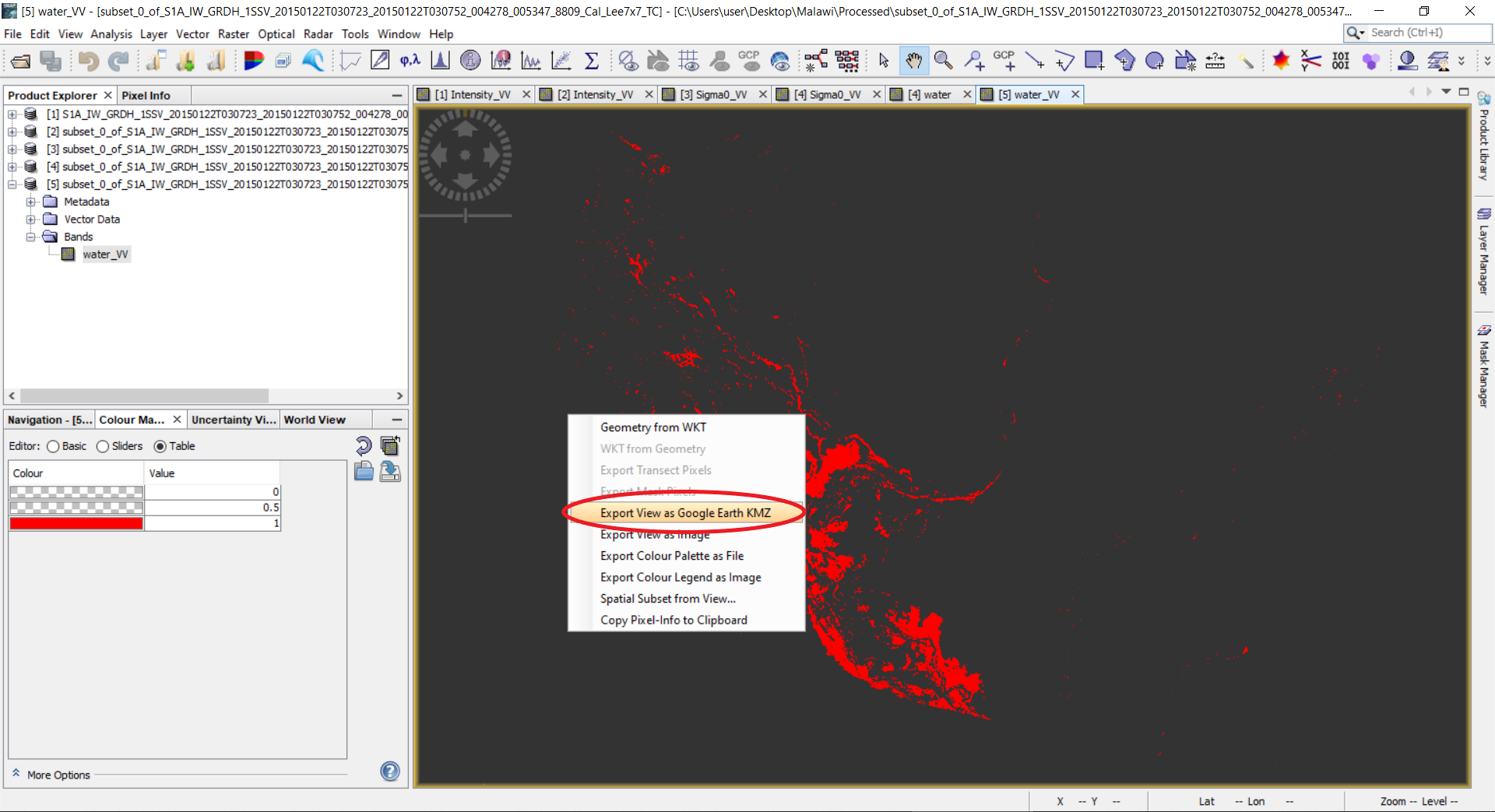
5.2 To visualize the water band in Google Earth, export it as a KMZ file; right click on the opened image --> Export View as Google Earth KMZ. Another way to export the flood mask is through File --> Export --> select file format to export.

5.3 Import the KMZ file to Google Earth.

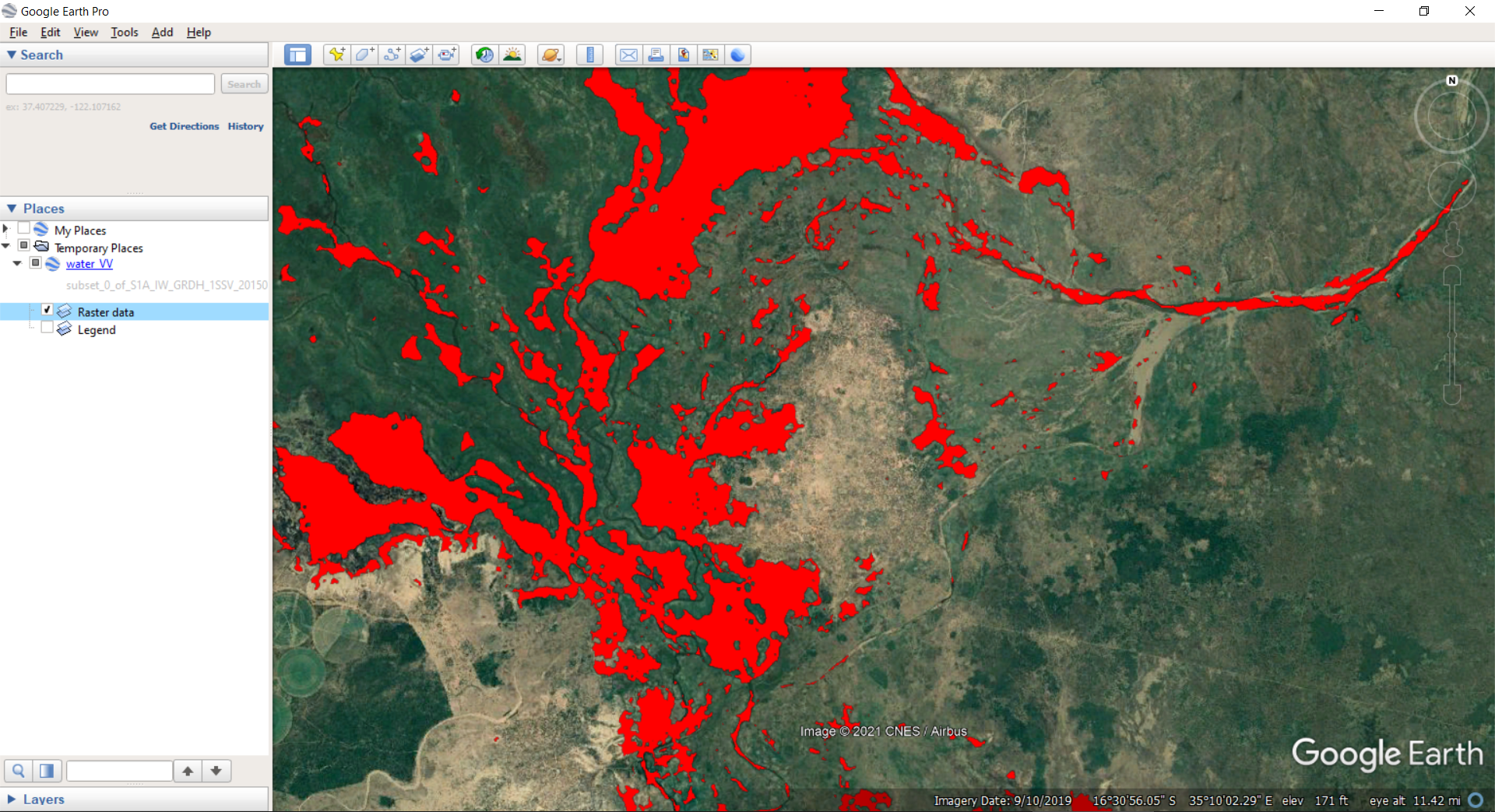
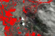
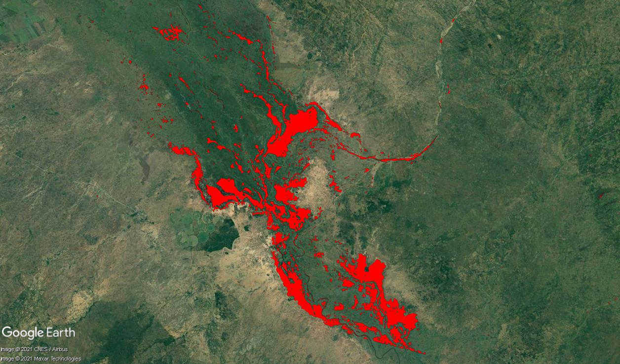
Example of the resulting product

Assessment

To assess the quality of the resulting flood mask, we compare it with the flood mask created by the Copernicus Emergency Management Service (EMS). The Copernicus EMS website for the flood event in Malawi (January 2015) can be found here and includes the results in vector format. These files can be imported and analyzed in a GIS (e.g., Quantum GIS).

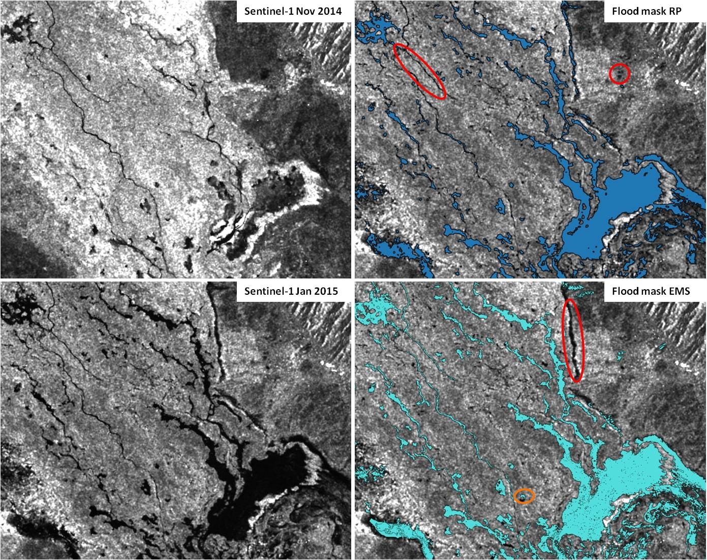
The following figure shows both flood masks in comparison. Due to the thresholding without manual post-editing or other post-processing techniques in the Recommended Practices Flood Mapping, several pixels around the main water bodies are found as water, whereby most of them might be false positives (a wrong classification of water). Apart from that and some river structures, there is an overall concordance between both flood masks.

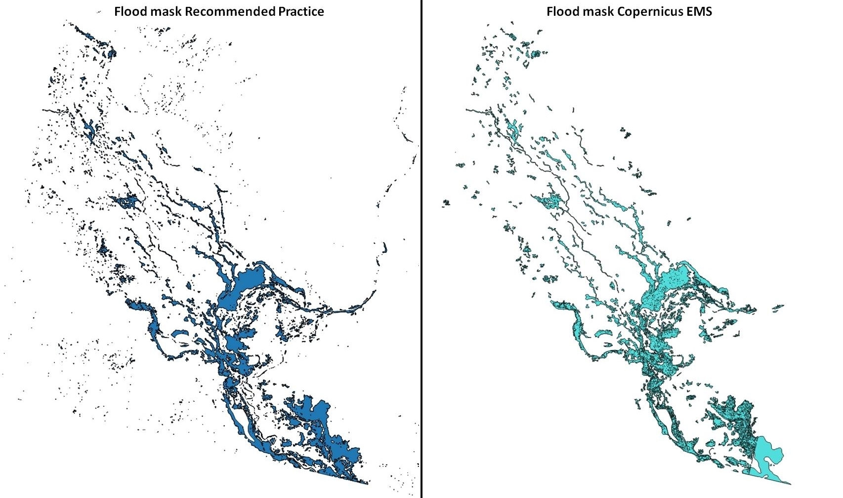
In the next figure Sentinel-1 subsets from before and during the flood event as well as the Recommended Practies and EMS flood masks are shown in detail. As an example, the red markings indicate false negatives meaning that water pixels were not classified as water. The orange marking of the EMS flood mask indicates an example for a false positive - a wrong classification of water.